

By Saad Iqbal
It’s the last week of the quarter and the reserves report is due Friday. Somewhere in a shared drive sits a spreadsheet with four thousand producing wells in it, and every one of them needs a decline curve refit before the numbers can be signed off. A reservoir engineer who is fast and careful can hand-fit maybe thirty wells a day — checking each Arps curve against the actual production history, nudging the decline exponent, flagging the wells where a recent workover or choke change makes the last six months of data lie about the well’s true decline. At thirty a day, four thousand wells is six months of work for a report that’s due in five days.
That arithmetic, more than any argument about model sophistication, is why machine learning decline curve analysis exists. The Arps hyperbolic equation that engineers have used since the 1940s hasn’t changed, and it doesn’t need to — what breaks down is the human workflow of fitting it well by well, catching the outliers by eye, and re-running the whole exercise every time new production data lands. ML-DCA automates that workflow, not the physics underneath it.
Why decline curve analysis doesn’t scale by hand
A clean decline curve analysis assumes clean data: a well that comes online, ramps briefly, then declines in a single smooth trend you can fit with one set of Arps parameters — initial rate qi, decline rate di, and the hyperbolic exponent b. Real production data almost never cooperates. Wells get choked back for pipeline curtailment, shut in for offset frac protection, worked over with a new artificial lift system, or simply report noisy daily volumes from a tank-battery allocation that smooths real variation into a sawtooth. Every one of those events creates either an outlier day that should be excluded from the fit, or a genuine change point where the well’s decline behavior shifts and the old curve stops applying.
An engineer doing this by eye on one well catches both in seconds — a glance at the production plot tells you where the workover bump is. The same judgment applied four thousand times, under a Friday deadline, is where human decline curve analysis quietly runs out of road.

What machine learning actually automates in decline curve analysis
The hyperbolic Arps equation stays exactly where it’s always been, at the center of the forecast. What a machine learning decline curve analysis pipeline adds is everything around that equation that used to require a trained eye:
- Outlier detection on daily or monthly volumes, typically using a rolling robust statistic or an isolation-forest style model, so a data-entry error or a single curtailed day doesn’t drag the fit off course.
- Change-point detection that flags where the well’s decline behavior genuinely shifts — a workover, an artificial lift conversion, or an offset frac hit — and segments the history so each regime gets its own curve instead of one curve straining to fit all of them.
- Automated non-linear regression that solves for qi, di, and b on each clean segment, often constrained to physically sensible ranges (b between 0 and 2 for most unconventional wells) so the solver doesn’t wander into a mathematically valid but geologically meaningless fit.
- A confidence or forecast-quality score per well, so engineers can triage: spend review time on the wells the model flags as uncertain, and accept the automated fit on the thousands it’s confident about.
- A rollup step that aggregates well-level EUR forecasts into type curves by area, vintage, or completion design — the number reserves and planning teams actually need.

Does machine learning replace the Arps equation?
No — and the tools built for this are explicit about that distinction. The Arps hyperbolic and exponential forms remain the forecasting model; what’s learned is which data points belong in the fit, where one decline regime ends and another begins, and how much weight to put on a forecast given how much clean history actually supports it. Some workflows pair Arps with a separate machine-learning layer that corrects for known biases — for instance, learning that wells in a given area tend to transition from hyperbolic to exponential decline earlier than a pure curve fit would suggest — but the underlying production-decline physics is the same equation reservoir engineers have run by hand for eighty years. If you want the mechanics of that equation itself, worked by hand, our step-by-step walkthrough of Arps decline curve analysis and EUR and fitting the Arps equation in Python both cover it from first principles.
A worked example: forecasting to the economic limit
Once a clean segment is isolated and qi, di, and b are fit, the forecast itself is the same hyperbolic Arps extrapolation it’s always been: rate declines forward in time until it crosses the well’s economic limit — the rate at which revenue no longer covers operating cost — and EUR is the cumulative volume produced up to that crossing point. What automation changes is how many times a day that forecast gets re-run as new production comes in, and how consistently the economic-limit rate itself gets applied across thousands of wells rather than being eyeballed per well.
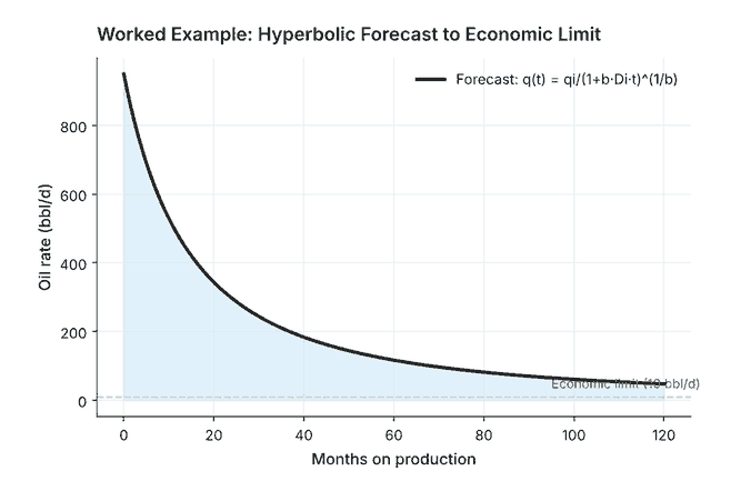
That consistency matters more than it sounds. A reserves book where one engineer applies a 10 bopd economic limit and another applies 5 bopd on comparable wells produces type curves that aren’t actually comparable, even though every individual fit was done carefully. An automated pipeline applies one rule everywhere, which means the variation left in the output reflects real differences between wells rather than differences between the engineers who fit them.
A pitfall automation won’t fix for you: allocated versus measured rates
There’s one data problem that outlier detection and change-point segmentation can’t solve on their own, because it isn’t noise in the usual sense — it’s a systematic artifact of how the volumes were measured in the first place. Most multi-well pads don’t meter every well continuously; they test each well periodically on a test separator and allocate the pad’s total metered volume back to individual wells by well-test ratio until the next test. A well’s daily “production” in the database is often an allocated estimate, not a measured rate, and every allocation method has its own bias.
Fed into a decline curve fit without adjustment, allocated volumes can manufacture a change point that isn’t real — a shift in allocation factors after a neighboring well comes online can look exactly like a genuine decline-rate change to a model that only sees the numbers. An automated pipeline that flags every allocation-driven step as a change point will over-segment the history and under-fit the true decline. The fix isn’t a smarter model; it’s tracing which wells on a forecast are allocated versus continuously metered before trusting a change point that lines up suspiciously well with another well’s startup date. This is the same allocation question that shows up in gas lift optimization at the field level, where injection-rate forecasting runs into an identical measurement problem from the other direction.
Tools built for this today
ComboCurve is built around exactly this workflow: it bulk-imports well data, auto-forecasts production at scale, and flags wells where actual production has diverged from the standing forecast so an engineer can review just those rather than the whole portfolio. Novi Labs’ Forecast Engine takes a different angle, pairing machine learning with geology, completion design, and well-spacing data to forecast not just producing wells but undrilled locations — useful for the planning side of the same reserves process. Neither tool is trying to out-think the Arps equation; both are trying to make running it four thousand times a week as reliable as running it once.
If decline curve analysis is new territory rather than a scaling problem, our roundup of AI reservoir simulation and forecasting tools is a reasonable next stop — it covers where DCA sits relative to full reservoir simulation, and when a type curve is enough versus when you actually need the physics-based model.
The equation didn’t get smarter. The workflow did.
It’s worth holding onto that distinction, because it’s easy to oversell this as the Arps equation finally being replaced by AI. It isn’t. What’s actually happened is that the parts of decline curve analysis that always relied on a trained eye — spotting the outlier, locating the change point, deciding when a curve is trustworthy enough to report — have been pulled into a pipeline that can run at the speed data actually arrives. For a four-thousand-well portfolio with a Friday deadline, that’s the difference that matters.
If you’re weighing whether to build this in-house or buy it, start smaller than the whole portfolio: pick fifty wells with known workover histories, run them through an automated change-point and Arps-fitting pipeline, and compare the segmented fits against what your engineers would flag by eye. That comparison tells you more about a tool’s real accuracy than any vendor demo will.
