Arps Decline Curve Analysis: EUR Step by Step

By Saad Iqbal

Ask three engineers to forecast the same well’s remaining reserves off the same production history and you’ll often get three different EUR numbers — not because the math is hard, but because the decline exponent b gets eyeballed, the decline rate’s time unit gets mixed up with the rate’s time unit, and nobody cross-checks the closed-form answer against a straight numerical integration of the curve. Arps decline curve analysis is one of the oldest tools in reservoir engineering precisely because it’s simple enough to do on a napkin — but that simplicity hides a unit-conversion trap that silently produces cumulative volumes that are an order of magnitude wrong. This tutorial builds the forecast by hand, verifies it two independent ways, and then automates it in Python.

What You’ll Need Before You Start

Step 1: Know the Governing Equations

Arps’ hyperbolic model describes production rate as a function of time with three parameters — qi, Di, and b:

q(t) = qi / (1 + b * Di * t)^(1/b)

Np(t) = [qi / (Di * (1 - b))] * [1 - (q(t) / qi)^(1-b)]

where
  q(t)  = rate at time t (same rate unit as qi, e.g. bbl/day)
  Np(t) = cumulative production from time 0 to t (rate-unit × time-unit)
  qi    = initial rate
  Di    = initial nominal decline rate (MUST be in 1/[time unit of t])
  b     = hyperbolic decline exponent, dimensionless
  t     = time since the start of the forecast

Two special cases fall out of the same formula: set b → 0 and it collapses to the exponential model q(t) = qi·exp(−Di·t); set b = 1 and it becomes the harmonic model q(t) = qi/(1 + Di·t). That’s a useful sanity check in itself — if your spreadsheet’s b = 0 case doesn’t match a hand-calculated exponential decline, the formula is wired up wrong before you’ve even gotten to the hyperbolic case.

Step 2: Watch the Unit Trap — Convert Di to the Same Time Base as t

This is where most hand calculations quietly break. Production software and decline-curve reports almost always quote Di as a percent-per-month or fraction-per-month figure, because that’s how field decline is usually eyeballed off a monthly allocation report. But if your rate qi is in bbl/day and you plug a monthly Di straight into the formula with t also in days, every cumulative-volume calculation downstream comes out roughly 30× too small — not obviously wrong, just quietly, confidently wrong. Convert first:

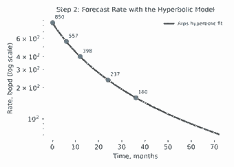
Di (per day) = Di_month (per month) / 30.4

Worked example: qi = 850 bopd, Di = 0.08/month (8% nominal monthly decline), b = 0.60, q_econ = 10 bopd. Converting: Di = 0.08 / 30.4 = 0.002632 per day. Running the rate equation with t in days and checking against a few calendar checkpoints:

Month	Rate (bopd)
0	850.0
6	557.5
12	398.3
24	237.0
36	159.6
60	88.7

Those rate checkpoints alone are the fastest way to catch the unit error: an 850 bopd well with an 8%/month nominal decline should still be making roughly 90 bopd five years in with b = 0.6 — if your version of this calculation shows single digits by month 24, the Di conversion is the first place to look.

Step 3: Integrate the Rate Curve to Get Cumulative Production

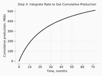
With Di correctly converted, the closed-form cumulative-production equation from Step 1 gives Np(t) directly in barrels (since qi is bopd and t is in days). Running it out to the same checkpoints:

Month	Cumulative Np (bbl)
6	125,373
12	211,236
24	323,051
36	393,901
60	480,470

Note this curve is still climbing at month 60 — the well hasn’t hit its economic limit yet at that point (see Step 4). The key validation step here is independent: integrate q(t) numerically with the trapezoidal rule over a fine time grid and compare it to the closed-form Np(t). In this example the two methods agree to within a few barrels out of over 670,000, which is the confirmation that the closed-form formula, the unit conversion, and the parameter values are all consistent with each other.

Step 4: Solve for the Economic Limit and EUR

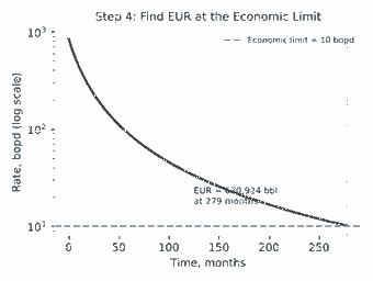
The well’s estimated ultimate recovery isn’t “cumulative production forever” — it’s cumulative production up to the day the rate drops to q_econ, the rate at which operating costs stop being covered by revenue. Because the hyperbolic rate equation is invertible, the time to reach q_econ has a closed form too:

t_econ = [ (qi / q_econ)^b − 1 ] / (b * Di)

Plugging in qi = 850, q_econ = 10, b = 0.60, Di = 0.002632/day: t_econ ≈ 8,472 days (≈ 278.7 months, ≈ 23.22 years). Evaluating Np at that time gives the well’s EUR ≈ 670,924 bbl — and because that number came from the same closed-form integral as Step 3, cross-checking it against the numerical trapezoidal integration out to t_econ is a one-line confirmation, not a separate calculation.

Step 5: Automate the Forecast and the Cross-Check in Python

Once the hand calculation checks out, there’s no reason to re-derive it by hand for the next well — wrap it in a function that takes the four parameters and returns the full table plus both validation checks:

import numpy as np

def arps_rate(t_days, qi, Di_day, b):
    if b == 0:
        return qi * np.exp(-Di_day * t_days)
    return qi / (1 + b * Di_day * t_days) ** (1 / b)

def arps_cumulative(t_days, qi, Di_day, b):
    if b == 0:
        return (qi / Di_day) * (1 - np.exp(-Di_day * t_days))
    q_t = arps_rate(t_days, qi, Di_day, b)
    return (qi / (Di_day * (1 - b))) * (1 - (q_t / qi) ** (1 - b))

def time_to_econ_limit(qi, Di_day, b, q_econ):
    if b == 0:
        return np.log(qi / q_econ) / Di_day
    return ((qi / q_econ) ** b - 1) / (b * Di_day)

# --- inputs ---
qi, Di_month, b, q_econ = 850.0, 0.08, 0.60, 10.0
Di_day = Di_month / 30.4

t_econ = time_to_econ_limit(qi, Di_day, b, q_econ)
EUR_closed_form = arps_cumulative(t_econ, qi, Di_day, b)

# independent numerical cross-check (trapezoidal integration)
tt = np.linspace(0, t_econ, 200_000)
qq = arps_rate(tt, qi, Di_day, b)
EUR_numerical = np.trapezoid(qq, tt)

print(f"t_econ          : {t_econ:,.0f} days ({t_econ/30.4:,.1f} months)")
print(f"EUR (closed form): {EUR_closed_form:,.0f} bbl")
print(f"EUR (numerical)  : {EUR_numerical:,.0f} bbl")

for m in [0, 3, 6, 12, 18, 24, 36, 48, 60, 72]:
    t = m * 30.4
    print(f"Month {m:3d}: rate = {arps_rate(t, qi, Di_day, b):7.1f} bopd   "
          f"cum = {arps_cumulative(t, qi, Di_day, b):10,.0f} bbl")

If you’d rather not re-implement Arps from scratch, the open-source petropt package ships a ready-made arps_decline function covering exponential, hyperbolic and harmonic cases, built on python.org‘s standard scientific stack. It’s a natural companion to a Z-factor or bubble-point-pressure workflow if you’re building a full reservoir-engineering toolkit rather than a one-off calculation.

Expected Result and How to Verify It

You should end up with a rate-vs-time table, a cumulative-production curve, a time to economic limit, and an EUR — and two independent confirmations that the number is right: the closed-form Np(t) should match a fine-grid trapezoidal integration of q(t) to within numerical noise, and the b = 0 case of your general hyperbolic function should match a hand-calculated pure-exponential decline exactly. If either check fails, the bug is almost always the Di time-unit conversion in Step 2, not the formula itself.

Three Pitfalls That Show Up on Location, Not on Paper

• Mixing Di’s time unit with t’s time unit. A Di quoted “per month” must be converted before it’s used with t in days, or cumulative volumes come out roughly 30× too small — always state which time base Di and t are in before writing a single line of code.
• Fitting b from too little or too noisy history. b is the hardest of the three parameters to pin down and the most sensitive to a short or choppy rate history; a few extra months of clean, representative data matters more than a more sophisticated fitting routine.
• Forgetting that b must stay in [0, 1] for a physically sensible hyperbolic decline. A fitted b outside that range (occasionally produced by an unconstrained least-squares fit) will still compute, but it no longer represents a decline mechanism grounded in the underlying physics.

A well’s actual decline shape is ultimately set by what’s happening in the reservoir — for a waterflood candidate, that means checking how close the front is to breakthrough with the Buckley-Leverett method before leaning too hard on a decline trend that’s about to change shape under injection.

Fitting a well that doesn’t behave like a clean hyperbolic? Share the shape of the problem in the comments — I read every one.