Gas Lift Valve Spacing: A Step-by-Step Design Method

By Saad Iqbal

An unloading program that doesn’t actually unload is one of the more expensive surprises in continuous-flow gas lift. The completion report shows twelve valves on paper, the well won’t kick off on location, and the first thing anyone reaches for is a wireline unit to pull and re-space the string — days of rig time to fix a spacing error that a half hour with a calculator would have caught. Valve spacing isn’t guesswork and it isn’t a vendor’s proprietary black box either: it’s two straight lines on a pressure-depth chart and one equation for the gas column between them. This tutorial walks through designing a full valve string by hand, then automates it in Python so you can re-run it in seconds every time the well’s gas-lift pressure or fluid gradient changes.

What You’ll Need Before You Start

Step 1: Plot the Kickoff and Operating Injection-Gas Lines

Every valve depth in the string comes from where two pressure-vs-depth lines cross, so the first job is drawing those lines correctly. The static gas column inside the tubing-casing annulus doesn’t follow a straight-line gradient the way a liquid does — gas compresses, so pressure builds with depth along a gentle curve. That curve is given by the standard static gas-column equation:

P(D) = Pio * exp[ 0.01875 * γg * D / (Z * Tavg) ]

where
  P(D) = gas pressure at depth D, psia
  Pio  = surface injection gas pressure, psia
  γg   = injection gas specific gravity (air = 1.0)
  D    = depth, ft
  Z    = average gas deviation (Z) factor, dimensionless
  Tavg = average gas column temperature, °R (°F + 460)

Run this equation twice — once with Pko (kickoff pressure) as Pio, once with Po (operating pressure) as Pio — and you get two curves: the kickoff line, used only to find Valve 1, and the operating line, used to space every valve below it. If your gas column’s average Z-factor is uncertain, the Dranchuk-Abou-Kassem correlation will get you a defensible number from gravity, pressure and temperature alone rather than an assumed 0.90.

Step 2: Find Valve 1 at the Kickoff/Unloading Intersection

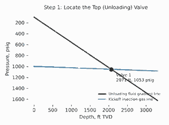
Valve 1 sits where the kickoff gas line crosses the unloading fluid gradient line — the line that starts at the wellhead unloading pressure and rises with the kill fluid’s gradient as you load the well down. Worked example, using a 7,000 ft packer, 100 psig unloading wellhead pressure, an 8.85-ppg (0.46 psi/ft) completion fluid, a 1,000 psig kickoff pressure, 0.65-gravity gas, 90°F surface / 170°F bottomhole temperature and Z = 0.90:

1. Unloading line: P(D) = 100 + 0.46·D (psig)
2. Kickoff gas line: P(D) = 1014.7·exp[0.01875·0.65·D / (0.90·Tavg(D))] − 14.7 (psig), with Tavg(D) interpolated linearly between 90°F at surface and 170°F at 7,000 ft
3. Stepping both lines down in 100 ft increments and bracketing the crossover, then bisecting, gives the intersection at approximately D₁ ≈ 2,071 ft, Pio ≈ 1,052.8 psig

That’s Valve 1: roughly 2,071 ft, set to open around 1,053 psig of injection gas pressure acting on the valve’s dome/bellows at that depth. Everything below it now follows the operating line, not the kickoff line, because once gas is injected at Valve 1 and unloading continues, the next valve down has to open against the lower, steady-state operating pressure — otherwise the whole string stays open simultaneously and you lose injection-gas efficiency.

Step 3: Space the Remaining Valves Down the Operating Line

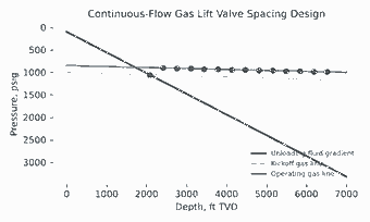
From Valve 1 down, each subsequent valve depth is found by intersecting the unloading fluid gradient (starting fresh from the previous valve’s opening pressure, decreased by your chosen design differential dP) with the operating gas line. In plain terms: you allow each valve to be dP psi “easier” to open than the one above it, draw a new fluid-gradient line through that lower pressure at the previous valve’s depth, and find where it meets the operating curve. Using dP = 150 psi for this completion, the first few valves come out at:

Valve	Depth (ft)	Injection Pressure (psig)
1	2,071	1,052.8
2	2,413	1,034.1
3	2,750	1,017.5
4	3,083	1,003.0
…	…	…
14 (operating)	6,521	991.8

Fourteen valves is not a typo and not over-design — it’s what falls out of the physics when the fluid gradient (0.46 psi/ft) is so much steeper than the gas column gradient. The two lines stay nearly parallel over most of the interval, so every 150 psi step in opening pressure only buys about 330–340 ft of additional depth. A shallower completion, a lower-gravity gas, or a larger dP would thin the string out; this one just needs that many valves to unload cleanly. The operating valve lands at 6,521 ft — about 479 ft of rathole standoff above the 7,000 ft packer, which is a comfortable margin for most completions.

Step 4: Size the Operating Valve’s Port With Thornhill-Craver

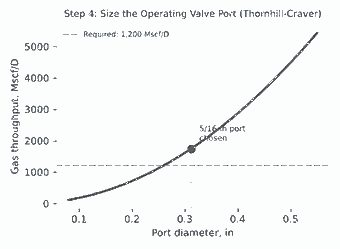
Spacing tells you where the operating valve sits; it says nothing about whether the port can actually pass your target injection-gas rate at the pressure differential available. That’s a separate, often-skipped check, and it’s where strings that unload perfectly on paper choke the well’s lift gas on location. The modified Thornhill-Craver orifice-flow equation gives the gas throughput through a given port size:

q = 155.5 * Cd * A * P1 * sqrt{ [2g*k / ((k-1)*Z*γg*T1)] * (r^(2/k) − r^((k+1)/k)) }

where
  q   = gas rate, Mscf/D
  Cd  = discharge coefficient (~0.865 for a square-edged port)
  A   = port area, in²
  P1  = upstream (casing) pressure, psia
  T1  = upstream gas temperature, °R
  k   = gas specific heat ratio (~1.28 for typical lift gas)
  g   = 32.17 ft/s²
  r   = P2/P1 (downstream/upstream pressure ratio), capped at the
        critical ratio rc = (2/(k+1))^(k/(k-1)) ≈ 0.552 for k = 1.28
        — flow is critical (sonic) below that ratio, so use rc instead

Worked example: the operating valve needs to pass 1,200 Mscf/D with P1 = 950 psia, P2 = 700 psia (r = 0.737, above rc so flow is subcritical — use the actual ratio), T1 = 630°R, γg = 0.65, k = 1.28, Z = 0.90, Cd = 0.865. Solving the equation for the required port area A and converting to diameter gives a required port of 0.2585 in. Round up — never down — to the nearest standard size, which is a 5/16-in (0.3125 in) port, rated for roughly 1,753 Mscf/D at those conditions: comfortable headroom over the 1,200 Mscf/D target without over-sizing to the point of poor pressure control.

Step 5: Automate the Full Design in Python

Hand-bisecting fourteen intersections is a fine way to learn the method once; it’s not how you want to re-run a design after the completion engineer changes the kickoff pressure for the third time. The same bisection logic above drops straight into a loop:

import math

def gas_column_psig(Pio_psig, D, gamma_g, Z, T_surf_F, T_bh_F, packer_D):
    Pio = Pio_psig + 14.7
    Tavg_R = (T_surf_F + (T_bh_F - T_surf_F) * D / packer_D) + 460
    return Pio * math.exp(0.01875 * gamma_g * D / (Z * Tavg_R)) - 14.7

def find_intersection(fluid_P0, Gu, Pio_psig, gamma_g, Z, Tsurf, Tbh, packer_D,
                       d_lo=0.0, d_hi=None, tol=0.05):
    d_hi = d_hi or packer_D
    f = lambda D: (fluid_P0 + Gu * D) - gas_column_psig(
        Pio_psig, D, gamma_g, Z, Tsurf, Tbh, packer_D)
    lo, hi = d_lo, d_hi
    while hi - lo > tol:
        mid = (lo + hi) / 2
        lo, hi = (lo, mid) if f(mid) > 0 else (mid, hi)
    return (lo + hi) / 2

# --- inputs ---
packer_D, Pwh, Gu  = 7000.0, 100.0, 0.46
Pko, Po            = 1000.0, 850.0
gamma_g, Tsurf, Tbh, Z = 0.65, 90.0, 170.0, 0.90
dP                  = 150.0

valves = []
d1 = find_intersection(Pwh, Gu, Pko, gamma_g, Z, Tsurf, Tbh, packer_D)
p1 = gas_column_psig(Pko, d1, gamma_g, Z, Tsurf, Tbh, packer_D)
valves.append((d1, p1))

fluid_P0 = p1 - dP
while valves[-1][0] < packer_D - 400:
    d_next = find_intersection(fluid_P0, Gu, Po, gamma_g, Z, Tsurf, Tbh,
                                packer_D, d_lo=valves[-1][0])
    p_next = gas_column_psig(Po, d_next, gamma_g, Z, Tsurf, Tbh, packer_D)
    valves.append((d_next, p_next))
    fluid_P0 = p_next - dP

for i, (d, p) in enumerate(valves, 1):
    print(f"Valve {i}: {d:7.0f} ft   {p:7.1f} psig")

def thornhill_craver_rate(Cd, d_in, P1_psia, P2_psia, T1_R, gamma_g, k=1.28, Z=0.90):
    A = math.pi / 4 * d_in**2
    rc = (2 / (k + 1)) ** (k / (k - 1))
    r = max(P2_psia / P1_psia, rc)
    g = 32.17
    term = (2 * g * k) / ((k - 1) * Z * gamma_g * T1_R)
    bracket = r ** (2 / k) - r ** ((k + 1) / k)
    return 155.5 * Cd * A * P1_psia * math.sqrt(term * bracket)

print(thornhill_craver_rate(0.865, 0.3125, 950, 700, 630, 0.65))

If you're scripting valve design regularly, the open-source petropt package wraps similar artificial-lift and PVT functions behind a cleaner API, and plugs straight into a nodal analysis model if you want to chase the full IPR-VLP-lift-curve loop in one script. The language itself is free — grab it from python.org if it isn't already on your machine.

Expected Result and How to Verify It

You should come out of this with a full valve schedule — depth, opening pressure and port size for every valve — that unloads progressively from the top down without ever opening two valves to atmosphere pressure at once. Verify it three ways before it goes to the completion crew: (1) confirm each valve's opening pressure decreases monotonically with depth; (2) check that the operating valve's port, run back through Thornhill-Craver at your actual available injection pressure and rate, clears your target gas rate with margin, not exactly at it; and (3) sanity-check the operating valve's standoff above the packer — you want enough rathole that a stuck or failed valve doesn't sit directly on top of the packer seal.

Three Pitfalls That Show Up on Location, Not on Paper

• Using a single average Z-factor for the whole column. Z changes meaningfully between surface and 6,000+ ft; if the margin on your design is thin, compute it at a few depth increments instead of one average value.
• Rounding the port size down "to save gas." A port sized at exactly the target rate leaves zero margin for a slightly colder morning or a slightly higher line pressure — round up to the next standard size every time.
• Ignoring the temperature gradient in the gas-column equation. Treating Tavg as a single surface temperature instead of interpolating to bottomhole temperature skews every intersection depth below it, compounding error down the string.

Once the string is spaced and sized, the next lever worth pulling is squeezing more barrels out of the same injection-gas budget — our guide to AI gas lift optimization software covers the tools now doing that allocation automatically across a pad.

Have a valve-spacing question specific to your completion? Drop it in the comments — I read every one.