

By Saad Iqbal
Your well is making 400 barrels a day, and the production meeting wants to know why it isn’t making more. The reservoir engineer says the rock can give you 1,200 barrels. The completions report says the tubing is fine. Nobody is lying — and yet the well sits at 400, stubbornly, day after day. Somewhere between the sand grains two miles down and the wellhead valve, a barrier is eating the difference. Finding it is not guesswork. It’s arithmetic you can do on one sheet of paper, and it’s called nodal analysis.
This is the same technique Carl Sagan might have reached for if he’d been handed a well file instead of a telescope: two independent descriptions of the same system — what the reservoir wants to deliver, and what the wellbore is willing to carry — plotted on the same axes until they agree. Where they cross is not a theory. It’s where your well actually lives.
What Nodal Analysis for an Oil Well Actually Solves
Nodal analysis for an oil well splits the flow path into two halves at a single point — usually the bottom of the tubing — and describes each half with its own curve. The inflow half is the reservoir: how much oil it will deliver at a given flowing bottomhole pressure, described by an Inflow Performance Relationship (IPR). The outflow half is everything above that point — tubing, wellhead choke, surface line — described by a Vertical (or Tubing) Lift Performance curve, VLP for short. Plot both as pressure versus rate, and the intersection is the only rate and pressure that satisfies both halves of the well at the same time. That intersection is the operating point. It’s the well’s actual answer, whether or not it’s the answer anyone wanted.
In this tutorial we’ll build the IPR with Vogel’s equation, build a simplified VLP curve by hand, find the operating point with one worked numeric example, and then hand the whole thing to a short Python script so you never have to re-derive it for the next well on your list.
Prerequisites — the sample values we’ll use throughout
Every number below recurs in every step, so the arithmetic stays traceable from the first equation to the last line of code. Swap in your own well-test data and the method doesn’t change.
- Average reservoir pressure, Pr = 2,500 psi
- Flowing bottomhole pressure during the test, Pwf,test = 2,000 psi
- Stabilized oil rate at that test point, qo,test = 400 STB/d
- Flowing wellhead pressure, Pwh = 150 psi
- Depth to mid-perforations (TVD), D = 8,000 ft
- Simplified flowing gradient, γ = 0.15 psi/ft
- Lumped tubing-friction coefficient, C = 0.0018 psi per (STB/d)²
That’s it — one stabilized flow test and four completion/surface numbers. No simulator required.
Step 1 — Build the Inflow Curve With Vogel’s IPR Equation
What to do: Vogel’s equation describes a solution-gas-drive reservoir’s inflow as a curved, bending-over relationship rather than a straight line. It is:
qo = qo,max × [ 1 − 0.2 × (Pwf / Pr) − 0.8 × (Pwf / Pr)² ]
- qo — oil rate at a given flowing bottomhole pressure (STB/d)
- qo,max — absolute open flow potential, AOF: the theoretical rate at Pwf = 0 (STB/d)
- Pwf — flowing bottomhole pressure at the sandface (psi)
- Pr — average reservoir (static) pressure (psi)
Why it matters: a straight-line Productivity Index (PI) assumes the well gets proportionally harder to produce as pressure drops — fine above the bubble point, wrong below it. Once free gas comes out of solution near the wellbore, it chokes the oil’s relative permeability, and the real curve droops faster than a straight line predicts. Vogel’s shape captures that droop with one dimensionless equation calibrated from a single flow test, which is exactly the data most wells already have sitting in a well-test report.
Worked example: we don’t know qo,max yet, but we know one point on the curve — the test point, Pwf,test = 2,000 psi, qo,test = 400 STB/d. Rearranging Vogel’s equation to solve for qo,max:
- Ratio = Pwf,test / Pr = 2,000 / 2,500 = 0.80
- Vogel fraction = 1 − 0.2(0.80) − 0.8(0.80)² = 1 − 0.16 − 0.512 = 0.328
- qo,max = qo,test / 0.328 = 400 / 0.328 = 1,220 STB/d (rounded)
That 1,220 STB/d is the absolute open flow — the ceiling the reservoir could theoretically deliver at zero bottomhole pressure. It is not a promise of what the well will actually produce; it’s one half of the equation. Plugging a range of Pwf values back into Vogel’s equation from 0 to 2,500 psi traces out the full IPR curve below.

Step 2 — Build the Outflow (VLP) Curve
What to do: the VLP curve answers the opposite question: for a given rate flowing up the tubing, how much pressure does the wellbore need at bottom to deliver it to surface against a fixed wellhead pressure? A full treatment uses a multiphase correlation — Hagedorn-Brown, Duns-Ros, or a mechanistic model — that accounts for slip, flow regime, and changing fluid properties with depth. For this tutorial we’ll use a deliberately simplified, honestly-labeled stand-in that keeps the shape and the teaching point without the correlation tables:
Pwf,vlp(q) = Pwh + γ × D + C × q²
- Pwf,vlp — flowing bottomhole pressure required to lift rate q (psi)
- Pwh — flowing wellhead pressure, held fixed by the choke/separator (psi)
- γ — simplified flowing gradient standing in for the gas-lightened fluid column (psi/ft)
- D — depth to mid-perforations (ft)
- C — lumped friction coefficient standing in for tubing friction losses (psi per (STB/d)²)
- q — oil rate flowing up the tubing (STB/d)
This is the honest caveat: real tubing performance isn’t a clean parabola. Slip between gas and liquid, flow-regime transitions (bubble to slug to mist), and changing PVT with depth all bend the real curve in ways a single q² term can’t fully capture. Treat this curve as the teaching skeleton of nodal analysis — the mechanics of finding an intersection — and swap in Hagedorn-Brown, Duns-Ros, or a vendor correlation once you’re sizing real equipment.
Why it matters: the hydrostatic term (γ × D) dominates at low rates — it’s the weight of the fluid column sitting in the tubing whether the well flows or not. The friction term (C × q²) is small at low rates but grows with the square of velocity, which is why VLP curves bend upward and eventually overwhelm any gain in rate: push too hard, and friction alone can demand more bottomhole pressure than the reservoir can supply.
Worked example: at q = 500 STB/d,
- Hydrostatic term = γ × D = 0.15 × 8,000 = 1,200 psi
- Friction term = C × q² = 0.0018 × 500² = 0.0018 × 250,000 = 450 psi
- Pwf,vlp = Pwh + 1,200 + 450 = 150 + 1,200 + 450 = 1,800 psi
Repeat that arithmetic across a range of rates from 0 to qo,max and you get the full VLP curve shown below — the pressure the wellbore demands to lift each possible rate to surface.

Step 3 — Find the Operating Point
What to do: plot the IPR and VLP curves on the same pressure-versus-rate axes. The reservoir’s IPR falls as rate rises; the wellbore’s VLP rises as rate rises. There is exactly one rate where the two curves cross — the only point where the pressure the reservoir is willing to deliver at the sandface exactly equals the pressure the wellbore needs to lift that same rate to surface. That crossing is the well’s operating point, and it’s where the well will actually sit, full stop, regardless of what anyone upstream of the choke was hoping for.
Why it matters: every lift-design decision — bigger tubing, gas lift, a bigger pump, a smaller choke — works by reshaping one of these two curves and sliding the intersection to a better rate. Nodal analysis is the tool that tells you, before you spend a dime on a workover, which curve is actually limiting you and by how much.
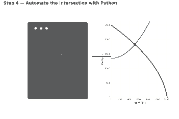
Worked example: solving the two equations simultaneously (or reading the crossing point off the two tables generated above) lands at approximately qo ≈ 517 STB/d at Pwf ≈ 1,832 psi. Check it: at Pwf = 1,832 psi, the IPR equation gives qo = 1,220 × [1 − 0.2(1,832/2,500) − 0.8(1,832/2,500)²] ≈ 518 STB/d. And at q = 517 STB/d, the VLP equation gives Pwf = 150 + 1,200 + 0.0018(517)² ≈ 1,831 psi. The two sides agree to within rounding — that’s the operating point.

Notice the gap: the reservoir could theoretically give 1,220 STB/d at Pwf = 0, but the wellbore only lets it deliver 517 STB/d. That gap between AOF and the operating rate is exactly what a lift-design engineer is paid to shrink — the same question answered quantitatively for an ESP well in our sucker rod pump volumetric efficiency walkthrough, and for a surface-choke-limited well in our choke size calculation with the Gilbert equation.
Step 4 — Automate Nodal Analysis With Python
What to do: hand-solving one well is a good way to learn the mechanics; running it on your next twenty wells is a job for a script. The code below rebuilds every number above — qo,max, the IPR array, the VLP array, and the intersection — using nothing but NumPy for the arrays and Matplotlib for the plot, found with linear interpolation so there’s no dependency on SciPy’s root-finder. Run it with Python directly, or paste it into a Jupyter notebook if you want to tweak the inputs interactively.
import numpy as np
import matplotlib
matplotlib.use("Agg")
import matplotlib.pyplot as plt

# ---- Reservoir / well-test inputs ----
Pr       = 2500.0   # psi, average reservoir pressure
Pwf_test = 2000.0   # psi, flowing BHP recorded during the test
qo_test  = 400.0    # STB/d, stabilized oil rate at Pwf_test

# ---- Tubing / surface inputs ----
Pwh   = 150.0   # psi, flowing wellhead pressure
depth = 8000.0  # ft, TVD to mid-perforations
grad  = 0.15    # psi/ft, simplified flowing (gas-lightened) gradient
C     = 0.0018  # psi per (STB/d)^2, lumped friction coefficient

# ---- Step 1: back out qo,max from the single test point (Vogel) ----
ratio = Pwf_test / Pr
qomax = qo_test / (1 - 0.2 * ratio - 0.8 * ratio ** 2)
print(f"qo,max (AOF) = {qomax:,.0f} STB/d")

# ---- Step 2: build the IPR curve ----
pwf_ipr = np.linspace(0, Pr, 400)
qo_ipr = qomax * (1 - 0.2 * (pwf_ipr / Pr) - 0.8 * (pwf_ipr / Pr) ** 2)

# ---- Step 3: build the VLP (tubing performance) curve ----
qo_vlp = np.linspace(0, qomax, 400)
pwf_vlp = Pwh + grad * depth + C * qo_vlp ** 2

# ---- Step 4: find the operating point (IPR x VLP intersection) ----
pwf_ipr_at_qvlp = np.interp(qo_vlp, qo_ipr[::-1], pwf_ipr[::-1])
diff = pwf_vlp - pwf_ipr_at_qvlp
idx = np.where(np.diff(np.sign(diff)) != 0)[0][0]
q1, q2 = qo_vlp[idx], qo_vlp[idx + 1]
d1, d2 = diff[idx], diff[idx + 1]
q_op = q1 - d1 * (q2 - q1) / (d2 - d1)
pwf_op = np.interp(q_op, qo_vlp, pwf_vlp)
print(f"Operating point: qo = {q_op:,.0f} STB/d at Pwf = {pwf_op:,.0f} psi")

# ---- Step 5: plot both curves and the operating point ----
plt.figure(figsize=(7, 5))
plt.plot(qo_ipr, pwf_ipr, label="IPR (Vogel)", linewidth=2)
plt.plot(qo_vlp, pwf_vlp, label="VLP (tubing)", linewidth=2)
plt.scatter([q_op], [pwf_op], color="red", zorder=5, label="Operating point")
plt.xlabel("Oil rate, qo (STB/d)")
plt.ylabel("Flowing bottomhole pressure, Pwf (psi)")
plt.title("Nodal Analysis: IPR vs VLP")
plt.legend()
plt.grid(alpha=0.3)
plt.tight_layout()
plt.savefig("nodal_analysis.png", dpi=150)
print("Saved plot to nodal_analysis.png")
Running this script prints qo,max (AOF) = 1,220 STB/d and Operating point: qo = 517 STB/d at Pwf = 1,832 psi — matching the hand calculation above exactly — and saves a chart of both curves with the operating point marked. If you’re batch-processing a field’s worth of wells from a spreadsheet of test data, pandas is the natural next step for looping this function over every row, and the open-source petropt package on PyPI collects several IPR/VLP correlations if you outgrow the simplified model here.
Sanity-Checking Your Result, and Common Pitfalls
Sanity check: three quick tests catch most mistakes before they reach a design meeting. First, qo,max should exceed your test rate by a believable margin, not an absurd one — a qo,max forty times the test rate usually means the test point was taken too close to Pr. Second, the operating rate should fall strictly between 0 and qo,max; if your “intersection” lands outside that range, one of the two curves was built with the wrong units or the wrong sign. Third, if the well has a surface choke or separator pressure reading, compare the model’s operating rate to the actual meter reading — they should agree within normal measurement scatter, not by an order of magnitude.
Common pitfalls:
- Using average or static pressure in place of flowing BHP. Vogel’s equation needs the pressure measured while the well was flowing at the test rate, not the shut-in reservoir pressure. Mixing the two silently shifts the whole IPR curve.
- Ignoring gas breakout and multiphase effects in the VLP. The simplified parabola here is a teaching tool. A well producing well below the bubble point, or with a changing gas-oil ratio, needs a real multiphase correlation before the VLP curve can be trusted for equipment sizing.
- Working from a stale well test. Reservoir pressure declines, water cut rises, and productivity index drifts over field life. An IPR built from a two-year-old test will quietly mis-locate every operating point you calculate from it — re-test, or at least re-anchor PI against recent production, before trusting the curve.
That gap between what the rock offers and what the wellbore allows through is the same gap decline-curve forecasting has to account for over the life of the well — worth a look in our decline curve analysis in Python piece if you want to see where this well’s rate is headed next year rather than just where it sits today.
Run this on your own well’s test data this week — the arithmetic takes ten minutes, and it’s usually the fastest way to find out whether a workover candidate is actually reservoir-limited or just needs a bigger straw.
