Natural Gas Z-Factor: The Dranchuk-Abou-Kassem Method

By Saad Iqbal

Pull a gas rate off a flow computer, plug it into a nodal model, a pipeline sizing sheet, or a material balance workbook, and the result is only as good as one number hiding inside almost every calculation you run on that stream: the natural gas Z-factor. Get it wrong by even a few percent and a gas well’s deliverability forecast, a gathering line’s pressure drop, or a reservoir’s OGIP estimate all drift with it. This tutorial builds the Z-factor calculation from gas specific gravity through to a converged value using the Dranchuk-Abou-Kassem (DAK) correlation — the same method running quietly inside most commercial PVT and nodal analysis software — with a verified worked example and a Python function you can drop into any script that needs real-gas behavior.

Prerequisites

Step 1: Convert Gas Gravity to Pseudo-Critical Properties

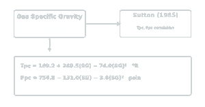
Z-factor correlations don’t work directly with pressure and temperature — they need those values normalized against the gas’s own critical point. Since a produced gas stream is a mixture, not a pure component, it doesn’t have a true critical point, so the industry uses pseudo-critical properties estimated from gas gravity. The Sutton (1985) correlation, fit to a broad set of sweet natural gas samples, gives:

Tpc (°R) = 169.2 + 349.5 × SG − 74.0 × SG²
Ppc (psia) = 756.8 − 131.0 × SG − 3.6 × SG²

Why it matters: every downstream step inherits whatever error shows up here. Sutton’s correlation is accurate to roughly ±1% on Tpc and ±2% on Ppc for sweet gas with SG between 0.57 and 1.68 — outside that range, or with significant non-hydrocarbon content, you need a compositional calculation or the Wichert-Aziz sour-gas correction instead.

Worked example: a gas stream with SG = 0.70, flowing at P = 2,000 psia and T = 150°F (610°R).

• Tpc = 169.2 + 349.5(0.70) − 74.0(0.70)² = 377.6 °R
• Ppc = 756.8 − 131.0(0.70) − 3.6(0.70)² = 663.3 psia

Step 2: Calculate Pseudo-Reduced Pressure and Temperature

With pseudo-critical properties in hand, reduce the actual flowing pressure and temperature against them:

Ppr = P / Ppc ​ ​ Tpr = T / Tpc

Why it matters: Ppr and Tpr are what the DAK correlation actually takes as inputs, and they’re also what tell you whether the correlation is even valid for your conditions — DAK is fit for 0.2 ≤ Ppr < 30 and 1.0 < Tpr ≤ 3.0. A gas stream near its critical point (Tpr close to 1.0 at low Ppr) sits in a region where Z changes fast with small pressure moves, and that’s exactly where a coarse correlation or bad pseudo-critical input does the most damage.

Continuing the example: Ppr = 2,000 / 663.3 = 3.015, and Tpr = 610 / 377.6 = 1.616. Both fall comfortably inside the DAK validity range.

Step 3: Solve the Dranchuk-Abou-Kassem Equation Iteratively

Z doesn’t fall out of a single formula — the DAK equation (1975) defines Z implicitly through the reduced gas density, so it has to be solved by iteration. The reduced density is:

ρr = 0.27 × Ppr / (Z × Tpr)

and the correlation itself is an 11-constant polynomial in ρr and Tpr:

Z = 1 + (A1 + A2/Tpr + A3/Tpr³ + A4/Tpr⁴ + A5/Tpr⁵)ρr + (A6 + A7/Tpr + A8/Tpr²)ρr² − A9(A7/Tpr + A8/Tpr²)ρr⁵ + A10(1 + A11ρr²)(ρr²/Tpr³)exp(−A11ρr²)

with coefficients A1–A11 = 0.3265, −1.0700, −0.5339, 0.01569, −0.05165, 0.5475, −0.7361, 0.1844, 0.1056, 0.6134, 0.7210.

Why it matters: guessing Z, computing ρr, recomputing Z, and repeating until the value stops changing is exactly what every PVT package does behind the scenes — understanding that loop is what lets you debug a spreadsheet that returns a nonsense Z, or extend the method to other correlations (Hall-Yarborough, Standing-Katz digitized charts) that share the same iterative structure.

Solving for the worked example (Ppr = 3.015, Tpr = 1.616) converges to Z = 0.833, with a reduced density ρr = 0.605 at convergence. At that Z, gas density works out to ρg = (28.97 × SG × P) / (Z × 10.732 × T) ≈ 7.44 lb/ft³, and the gas formation volume factor Bg = 0.02827 × Z × T / P ≈ 0.00718 rcf/scf — both numbers you’d otherwise have pulled off a Standing-Katz chart by eye.

Step 4: Sanity-Check Against the Shape of the Standing-Katz Chart

Before trusting a computed Z-factor, check that it’s at least shaped right. Z starts near 1.0 at low pressure (ideal-gas behavior), dips to a minimum somewhere in the Ppr = 1–3 range as attractive molecular forces dominate, then climbs back above 1.0 at high pressure as molecular volume effects take over. Higher Tpr curves sit higher on the chart and dip less sharply.

Why it matters: this is the fastest way to catch a unit error or a bad pseudo-critical input before it propagates into a rate or reserves number. A computed Z above 1.2 at moderate pressure, or below 0.5, usually means Ppr or Tpr was built with the wrong units (psig instead of psia is the classic one) rather than a real gas property.

Our worked example’s Z = 0.833 at Tpr = 1.616, Ppr = 3.015 sits right in the expected dip region for a mid-Tpr curve — consistent with the shape, and a reasonable value for a moderate-gravity gas at these conditions.

Step 5: Automate It With Python and SciPy

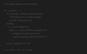
Hand iteration is fine once; a function is better for every well test, every day of pipeline flow data, or every point on a gas deliverability curve. SciPy‘s brentq root finder handles the implicit solve in a few lines:

from scipy.optimize import brentq
import math

A = [0.3265, -1.0700, -0.5339, 0.01569, -0.05165,
     0.5475, -0.7361, 0.1844, 0.1056, 0.6134, 0.7210]

def z_dak(Ppr, Tpr):
    def residual(z):
        rr = 0.27 * Ppr / (z * Tpr)
        z_calc = (1
            + (A[0] + A[1]/Tpr + A[2]/Tpr**3 + A[3]/Tpr**4 + A[4]/Tpr**5) * rr
            + (A[5] + A[6]/Tpr + A[7]/Tpr**2) * rr**2
            - A[8] * (A[6]/Tpr + A[7]/Tpr**2) * rr**5
            + A[9] * (1 + A[10]*rr**2) * (rr**2/Tpr**3) * math.exp(-A[10]*rr**2))
        return z_calc - z
    return brentq(residual, 0.3, 3.0, xtol=1e-10)

def pseudocritical(sg):
    tpc = 169.2 + 349.5*sg - 74.0*sg**2   # degR, Sutton 1985
    ppc = 756.8 - 131.0*sg - 3.6*sg**2    # psia
    return tpc, ppc

sg, p_psia, t_rankine = 0.70, 2000.0, 610.0
tpc, ppc = pseudocritical(sg)
ppr, tpr = p_psia/ppc, t_rankine/tpc
z = z_dak(ppr, tpr)
print(f"Tpc={tpc:.1f} R, Ppc={ppc:.1f} psia, Ppr={ppr:.3f}, Tpr={tpr:.3f}")
print(f"Z = {z:.4f}")
# Tpc=377.6 R, Ppc=663.3 psia, Ppr=3.015, Tpr=1.616
# Z = 0.8333

Vectorize the same function over a pandas DataFrame of daily flowing pressures and temperatures and you get a running Z-factor and gas density series for free — feed that straight into the gas rate equation behind a gas gathering line sizing calculation, a nitrogen volume calculation for a coiled tubing job, or the P/Z term in a gas reservoir material balance — every one of them needs exactly this Z-factor as an input.

Expected Result and Common Pitfalls

You should come away with a converged Z-factor for your gas and conditions, confidence that it falls in a physically reasonable range for the pseudo-reduced properties involved, and a reusable function for the next hundred data points. Verify a hand or script result against a digitized Standing-Katz chart reading at the same Ppr and Tpr — DAK should track within about 0.5% of the chart across its valid range.

• Mixing psig and psia. Pseudo-critical pressure and Ppr are defined in absolute units. Forgetting to add atmospheric pressure to a gauge reading silently shifts every downstream number.
• Applying Sutton’s sweet-gas correlation to sour gas. H2S and CO2 both shift the true critical point; above a percent or two of either, apply the Wichert-Aziz correction to Tpc and Ppc before computing Ppr and Tpr, or the DAK solve will converge to a confidently wrong answer.
• Starting the iteration far from the root with a tight bracket. If brentq raises a sign-error instead of converging, the true Z likely sits outside the [0.3, 3.0] bracket — widen it, and double-check Ppr/Tpr are in the valid DAK range before assuming the correlation itself is at fault.