

By Saad Iqbal
An ESP running a mid-continent oil well has been sitting at 42 Hz for eleven months, making 310 bbl/day without complaint. Then its radial vibration starts a slow, almost imperceptible climb — a tenth of a millimeter per second here, another tenth there. The fixed-threshold alarm on the SCADA screen stays green the entire time, because it’s tuned to catch a sudden spike, not a creeping drift. Three weeks later the string trips on high vibration, the well goes dark, and a workover rig gets a call it could have gotten two and a half weeks earlier. This is the exact failure mode AI ESP failure prediction was built to close, and the industry has spent three years proving the concept works. What’s changed more recently is subtler and, for anyone actually running a fleet of pumps, more useful: the output is no longer a single red flag. It’s a curve.
The Trouble With a Single Alarm Threshold
A fixed threshold is a blunt instrument because it has to be. Set it too tight and every well with slightly thicker fluid or a slightly worn bearing trips a false alarm on a Tuesday afternoon. Set it loose enough to avoid nuisance trips and you’ve just guaranteed the alarm fires close to the actual failure, which is to say, too late to matter. Thresholds also can’t distinguish between a vibration signature that means “bearing wear, six weeks of life left” and one that means “shaft misalignment, six hours of life left.” They’re a tripwire, not a diagnosis.
The alternative that’s matured over the last few years treats the sensor stream as a classification and regression problem instead of a tripwire. A model trained on run-to-failure history from hundreds or thousands of ESP strings learns what the data looks like in the weeks before a bearing wears out, a shaft misaligns, a seal section floods, or free gas starts locking a stage — and scores every new reading against those learned signatures rather than one static number.
Where an AI ESP Failure Prediction Model Actually Taps the String
None of this works without data the industry was already collecting, mostly for other reasons. A modern ESP installation runs a downhole gauge — a Phoenix-type sensor package is the generic shorthand — reporting motor winding temperature, radial and axial vibration, intake and discharge pressure, and fluid frequency drift back to the variable speed drive every minute. Motor current and load come from the drive itself. None of it was installed for AI; it was installed so an operator could see the well was still running. The prediction layer just asks a harder question of data that was already there.
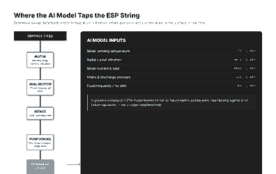
What changes between a basic alarm and a genuine prediction model is what happens to those five or six signal streams once they leave the gauge. A gradient-boosted model, or increasingly an LSTM trained on sequences rather than single readings, isn’t looking for one value crossing one line. It’s looking for the shape of the multivariate drift — vibration rising while temperature holds steady points one direction, temperature and current rising together points another — and matching that shape against failure modes it has seen before.
The Window Between Drift and Trip
The illustration below is a composite, not one specific well’s telemetry, but it draws the shape correctly: a vibration trend that would sit comfortably inside a “normal operating band” for most of its life, rising gradually enough that a fixed threshold doesn’t fire until day 31, the day of the trip. A model trained on prior failure sequences on that same string — or, more realistically, on a population of similar strings — flags the same drift around day 14, roughly two weeks earlier. That gap is the entire value proposition. It’s the difference between an emergency callout and a workover scheduled on your terms, with a rig and a pulling unit lined up instead of a well sitting dead for however long it takes one to become available.

Turning a Trend Line Into a Remaining-Useful-Life Curve
Here’s where the last couple of years have actually moved the needle, and it’s a statistical shift more than a sensor one. Reliability engineers have used survival analysis — Weibull hazard functions, in particular — to describe time-to-failure for rotating equipment for decades, mostly at the fleet level: a Weibull shape parameter above 1 tells you failure rate increases with age, which is exactly what wear-out mechanisms like bearing degradation do. What’s changed is applying that same framework per well, continuously, conditioned on live sensor drift rather than just elapsed run time.
Practically, that means the model’s output stops being a binary “healthy / at risk” flag and becomes a remaining-useful-life estimate with a confidence band — something closer to “60% probability of failure within 21 days, rising to 85% by day 35” than a single tripwire. That’s a genuinely different artifact to hand a production engineer. A binary flag asks you to trust a black box. A RUL curve with a confidence band lets you weigh the cost of a false positive against the cost of a missed failure using numbers you can defend in a budget meeting, and it updates every time new telemetry comes in instead of staying fixed until the next model retrain.
What the Published Numbers Actually Say
It’s worth being precise about what’s actually been documented publicly, because vendor marketing in this space tends to round up. Three figures are worth anchoring to:

- 92% precision. GeoPark’s Colombian ESP program, running AI analytics built with Halliburton, reports predicting ESP failures with 92% precision — a published figure, not a rounded marketing claim.
- 38% run-life improvement. SLB has documented a 38% ESP run-life gain from a program combining extended-life pump hardware with a chemical treatment regime. Worth flagging honestly: that’s a hardware-and-chemistry result, not a pure analytics one, so it belongs in the conversation as a run-life benchmark rather than proof that AI alone delivers 38%.
- $8 million saved. Baker Hughes’ permanent failure analysis program on a European offshore asset is credited with $8 million in avoided failure costs — the kind of number that survives scrutiny because it’s tied to a named deployment rather than an industry average.
None of those numbers transfer directly to your field. Failure economics depend on workover rig availability, deferred-production value at current pricing, and how many strings you’re running. But they’re real anchors, and they’re more useful than the unsourced “150% improvement” figures that circulate in slide decks without a case study behind them.
Building the Business Case Without Overselling It
The honest pitch to a production manager isn’t “AI will stop your ESPs from failing.” ESPs fail; that’s baked into the hardware. The honest pitch is that the failure stops being a surprise. A string that was going to trip on a Tuesday night now trips on a forecast, two to three weeks out, with enough lead time to stage a pulling unit, order the replacement pump, and schedule the workover for daylight hours instead of an emergency callout. Run that math across a fleet of fifty or a hundred ESP wells and the deferred-production savings compound fast, even before you account for the rig trips that get combined instead of run one at a time.
Where This Fits Against Other Lift Methods
ESPs got AI attention early, in part because electrical signals are easy to instrument and because the failure cost per well is high enough to justify the investment. Other lift methods are catching up at different speeds. Jet pumps are still mostly tuned manually, a genuine gap given how little hardware instrumentation they need to close it. Progressive cavity pumps have their own three-signature failure pattern — wear, elastomer swelling, gas interference — readable from torque, speed and flow alone, no new gauge required. And the foundational case for doing any of this on ESPs specifically was covered here in detail when motor current signature analysis was the newer idea; the RUL-curve approach above is the natural next step past that baseline.
What to Actually Do With This Monday Morning
You don’t need a six-figure platform contract to start getting value out of this logic. If your downhole gauges and VSD already log vibration, temperature, current and pressure to a historian — and on most modern ESP installations they do — a rolling 30-day baseline per well, with drift flagged as a percentage deviation from that baseline rather than a fixed absolute number, catches the same early signal a vendor platform would, just with less precision about which failure mode is coming. That’s not nothing. It’s the difference between finding out your well tripped and finding out it’s drifting, which is the entire point. Start there, watch which wells actually drift ahead of a real failure, and you’ll have a far better case — built on your own field’s data instead of someone else’s — for whether the next step is a vendor contract or an in-house model.
