

By Saad Iqbal
Watch a casing pressure trend on an unstable gas-lifted well for a few hours and you’ll see the same pattern every time: pressure climbs, climbs, climbs — then collapses in a matter of minutes, production surges in a slug, and the whole cycle starts again. That’s casing heading, and by the time it shows up clearly on a trend screen, you’ve usually already lost weeks of production to it. AI gas lift instability detection exists to catch that cycle in its first few hours instead of its fifth day — flagging the signature in the pressure data before an operator would ever notice it by eye, and triggering a choke adjustment before the well settles into a chronic slugging pattern.
This is a mechanical problem with a mechanical fix — trim the injection choke — but the hard part has never been the fix. It’s catching the instability early enough, and consistently enough across a big gas-lift portfolio, that someone actually acts on it. That’s exactly the kind of pattern-recognition-at-scale problem a fairly simple classifier handles well. Here’s the full build.
What Is Casing Heading, and Why Does It Cost You Barrels?
In a continuous gas-lift well, injection gas is supposed to move steadily from the casing annulus, through the gas lift valve (GLV), into the tubing — lightening the fluid column and helping it flow. Casing heading happens when that handoff isn’t steady: gas accumulates in the annulus faster than it can bleed through the GLV, annulus pressure builds, and once it finally overcomes the valve’s opening pressure, a large slug of gas dumps into the tubing all at once. That slug unloads liquid ahead of it, tubing pressure spikes then collapses, casing pressure craters because it just dumped its stored gas, and the cycle resets to start climbing again.
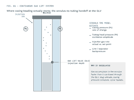
The production hit isn’t subtle. Cyclic slugging means you’re periodically over-lifting (wasting compression gas) and then under-lifting (the well briefly loads up before the next slug clears it), and neither extreme is anywhere near the well’s optimal lift-gas rate. Depending on how severe the cycle is, published field studies put the production loss anywhere from single digits to over 20% versus a stabilized well on the same average gas injection rate — which means the fix isn’t just about smoother trends, it’s leaving real barrels on the table every day it runs uncaught.
The Signals That Give Casing Heading Away Before an Operator Notices
An experienced production engineer can spot heading on a trend screen, but by the time it’s visually obvious the well has usually been cycling for a while. The signals that catch it earlier are the same pressure and rate tags most gas-lift wells already stream to SCADA — you’re just looking at them differently:
- Casing pressure (Pc) rate of change. A healthy well shows small, high-frequency noise. A heading well shows a slow, large-amplitude ramp — the signature you want to catch is the ramp rate exceeding a threshold, not the absolute pressure.
- Tubing head pressure (Pt) oscillation amplitude. This is the downstream symptom — the slug arriving. Amplitude and period both matter; a shortening period on successive cycles is often a sign the instability is worsening.
- Injection gas rate versus set point. If the actual injection rate is swinging around the choke’s target instead of holding steady, that’s the annulus alternately accepting and then dumping gas.
- Dominant oscillation frequency from a rolling FFT on the pressure signal — casing heading has a fairly characteristic period (often tens of minutes to a couple of hours depending on annulus volume and GLV port size), distinct from the high-frequency noise of normal operation or the very slow drift of a genuine reservoir-pressure decline.
None of these individually is a reliable trigger — a single pressure spike could be a slug catcher dump or a choke change, not instability. It’s the combination, sustained over a rolling window, that separates real heading from noise.
How to Build an AI Model That Flags Instability in Real Time
This is a classification problem, not a regression one: at any given moment, is this well stable or heading? A gradient-boosted tree classifier (the same family that works well for the wax deposition problem covered in our AI dynacard diagnostics piece) trained on rolling-window features tends to outperform a simple fixed-threshold alarm, because it can combine several weak signals instead of relying on any one of them crossing an arbitrary line.
The feature-engineering step is where most of the value gets built: take the raw 1 Hz (or whatever your polling rate is) casing and tubing pressure tags, and compute rolling statistics over a window — standard deviation, rate of change, and the FFT-derived dominant frequency and its magnitude — rather than feeding raw pressure into the model. Raw pressure varies well-to-well with depth and reservoir pressure; the shape of the oscillation is what generalizes across a portfolio. Label the training data using historical incidents your team already logged (or, if you don’t have clean labels yet, start with a simpler rule-based flag — sustained Pc ramp plus Pt oscillation above a threshold — use it to bootstrap labels, then retrain the classifier on top of it once you’ve accumulated confirmed events).
A Worked Example: From Raw Pressure Data to an Automated Choke Trim
Here’s what this looks like on an actual well over a six-hour window. Casing pressure is cycling between roughly 380 and 590 psi with a period of around 25–30 minutes — a clean casing-heading signature. At the 3-hour-24-minute mark, the model’s rolling features cross its trained decision boundary, an alert fires, and (in this case) an automated choke trim reduces the injection rate slightly to break the cycle.

The oscillation doesn’t vanish instantly — there’s a damping period of roughly ninety minutes as the annulus and tubing find a new equilibrium, which is normal and expected for a step change in injection rate. What matters is the trend: amplitude decaying cycle over cycle rather than sustaining or growing. If a trim doesn’t produce that decay pattern within a similar window, that’s itself a useful signal — it suggests the instability isn’t simple casing heading and needs an engineer to look at valve condition, injection point depth, or a genuine mechanical issue rather than another automated trim.
What Happens After Detection: Automating the Response
Detection without action is just a prettier trend chart. The full pipeline runs in four stages, from raw tag to response:

Whether stage four is a fully automated choke trim or an alert routed to an engineer for manual approval is a judgment call most operators should make conservatively at first — automate the alert before you automate the actuation. A Python service scoring the classifier on a rolling basis can write flagged events to a shared table; a no-code flow in Make, n8n, or Power Automate watches that table and pushes a Slack or Teams alert with the well name, the flagged window, and a link to the trend. Once you’ve built confidence in the classifier’s precision on your specific field — field trials on this kind of model commonly report false-positive rates held under 4–5% with a well-tuned rolling window — moving to an automated choke trim through your existing SCADA/PLC integration is a smaller step.
Tools for Building This Yourself
- Python with pandas for the rolling-window feature engineering (standard deviation, rate of change, FFT) on the raw pressure tags.
- petropt for the underlying artificial-lift and multiphase-flow correlations if you want to extend the model with physics-based features like predicted GLV performance at current conditions.
- Microsoft Power BI or Google Looker Studio for a portfolio-wide dashboard so a production engineer can see every well’s current stability status at a glance, not just the one that just alerted.
- Make, n8n, or Power Automate to turn a classifier flag into a routed alert or an automated choke command.
- Claude or ChatGPT for drafting the FFT feature code, explaining an unfamiliar valve spec sheet, or writing the incident summary an engineer has to file after a confirmed heading event.
Common Pitfalls Worth Knowing Before You Build This
- Confusing casing heading with density-wave or slug-flow instability further up the tubing. Both produce cyclic tubing pressure, but the fix is different — a casing heading model that only looks at Pt in isolation, without the casing-side signal, will mis-classify the two.
- Training on too short a history. Casing heading period scales with annulus volume, which varies well to well — a model trained on one field’s typical 20–30 minute cycles may need retuning for a field with much larger annulus volumes and multi-hour cycles.
- Automating the trim before validating precision. A false positive that trims a genuinely stable well’s injection rate costs production for no reason — get comfortable with the alert-only stage first, the way you’d validate any new automated control action.
The upside case here is real and it’s not exotic: this is the same rolling-features-plus-classifier pattern used across artificial lift diagnostics generally, including the rod-pump dynacard work and ESP failure prediction we’ve covered previously — different failure signature, same underlying approach of turning a raw sensor stream into an early, automatable flag.
