
By Saad Iqbal
A completions team spends extra proppant mass packing a short fracture wide and conductive, expecting a stronger well. The frac job goes exactly to plan — tight tolerances, good near-wellbore conductivity, clean treating pressure. Three months later the type curve undershoots the offset wells. Nothing went wrong on location; the design itself was aimed at the wrong target. The fracture was already far more conductive than the reservoir needed, and the same proppant, spread into a longer fracture instead, would have contacted more rock and produced more oil.
That failure mode has a name and a number attached to it: dimensionless fracture conductivity, usually written CfD. It tells you whether a frac design is conductivity-limited, length-limited, or already balanced — and paired with the proppant number, it tells you how to fix a design that’s out of balance, using the proppant you already planned to pump. This tutorial walks through calculating CfD, checking it against the proppant number rule, and resizing a real design to its optimum.
Prerequisites
- Formation (matrix) permeability, k — here: 0.1 md (a tight unconventional reservoir).
- Proppant-pack permeability, kf — here: 20,000 md, a representative value for 20/40 sand at moderate closure stress.
- Planned propped fracture half-length, xf — here: 80 ft.
- Planned propped fracture width, w — here: 0.10 in.
- Pay (net) thickness, h — here: 100 ft.
- Drainage area side length, xe — here: 2,640 ft (a square 160-acre spacing unit).
- A way to run a short Python script (or a spreadsheet) for the resizing step.

Step 1 — Lay Out the Frac Geometry and Reservoir Inputs
Dimensionless fracture conductivity compares how easily fluid moves along the fracture to how easily it moves into the fracture from the reservoir. That means it needs both a fracture description (permeability and width of the propped pack) and a reservoir description (matrix permeability and how big a drainage area the fracture has to serve). Lay out the well on 160-acre spacing — a square drainage area with side length xe = 2,640 ft — with a planned fracture half-length of 80 ft reaching out from the wellbore at the center.
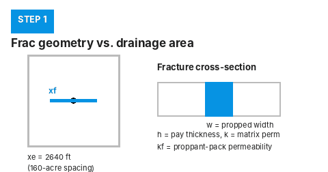
Why it matters: every term in the conductivity and proppant-number equations below comes straight from this geometry. Get xf, w, k, kf, h, and xe pinned down correctly here and the rest is arithmetic.
Step 2 — Calculate Dimensionless Fracture Conductivity, CfD
The governing equation (Cinco-Ley and Samaniego; the standard form used in unified fracture design) is:
C_fD = (kf × w) / (k × xf)- kf = proppant-pack permeability, md
- w = propped fracture width, ft
- k = formation permeability, md
- xf = propped fracture half-length, ft
Converting width to feet (0.10 in = 0.00833 ft) and plugging in:
C_fD = (20,000 × 0.00833) / (0.1 × 80)
C_fD = 166.7 / 8
C_fD = 20.8
Why it matters: a fracture is considered finite-conductivity (bilinear flow dominates early time) below roughly CfD = 100, and high-conductivity (acts almost like an infinite-conductivity fracture) at or above it. Our value of 20.8 sits comfortably in finite-conductivity territory — not high enough to ignore, but that alone doesn’t tell us whether 20.8 is the right number for this well. For that we need the proppant number.
Step 3 — Calculate the Proppant Number and Apply the Optimum-CfD Rule
Unified fracture design links CfD to a second dimensionless group, the proppant number, which measures how much propped fracture volume you’re putting into the reservoir relative to the reservoir volume the fracture has to drain:
Ix = 2·xf / xe              (penetration ratio)
Nprop = Ix² × C_fD           (proppant number)
For our design: Ix = 2 × 80 / 2,640 = 0.0606, so Ix² = 0.00367, and:
Nprop = 0.00367 × 20.8 = 0.0765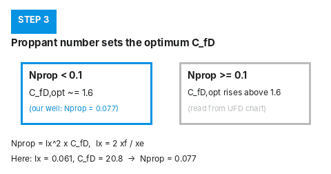
This is the key decision rule from unified fracture design: for Nprop below 0.1, the optimum dimensionless conductivity that maximizes productivity is CfD,opt ≈ 1.6, regardless of how much higher the as-designed CfD is. Above Nprop = 0.1, the optimum CfD rises (because the penetration ratio can’t exceed 1), and reading it off requires the full optimization chart rather than a single number. Our well’s Nprop = 0.077 falls below 0.1 — so the 1.6 rule applies directly, and our as-designed CfD of 20.8 is more than twelve times higher than it needs to be. Why it matters: this is the signal that the job is over-conductive and under-penetrated — the same proppant would do more good spread further out.
Step 4 — Resize the Fracture to the Optimum Design
Keep the propped volume fixed (same proppant mass pumped) and re-solve for the xf and w that hit CfD,opt = 1.6 instead. The propped volume for both wings is:
Vprop = 2 × w × h × xf
Vprop = 2 × 0.00833 × 100 × 80 = 133.3 ft³
Combining Vprop = 2·w·h·xf with CfD,opt = kf·w / (k·xf) and solving for xf gives the optimum half-length directly:
xf_opt = √( Vprop × kf / (2 × C_fD,opt × k × h) )
xf_opt = √( 133.3 × 20,000 / (2 × 1.6 × 0.1 × 100) )
xf_opt = √83,312 ≈ 289 ft

w_opt = C_fD,opt × k × xf_opt / kf
w_opt = 1.6 × 0.1 × 289 / 20,000 ≈ 0.0023 ft ≈ 0.028 in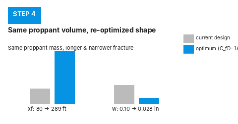
Why it matters: the same proppant mass, pumped to a half-length of about 289 ft at a width of about 0.028 in instead of 80 ft at 0.10 in, puts the design back on the optimum CfD = 1.6 curve — more reservoir contact, same cost, no extra proppant.
Automate It With Python
This function runs the full check — CfD, proppant number, and the resized geometry — on any set of inputs:
# Requires: Python 3 (https://www.python.org)

def frac_conductivity_check(k, kf, xf_ft, w_ft, h_ft, xe_ft, cfd_opt_low_nprop=1.6):
    """Returns CfD, proppant number, and an optimum-CfD resize
    for a fixed propped volume, per unified fracture design."""
    cfd = (kf * w_ft) / (k * xf_ft)
    ix = (2 * xf_ft) / xe_ft
    nprop = ix ** 2 * cfd

    vprop = 2 * w_ft * h_ft * xf_ft  # both wings, ft^3

    result = {"CfD": cfd, "Ix": ix, "Nprop": nprop, "Vprop_ft3": vprop}

    if nprop < 0.1:
        cfd_opt = cfd_opt_low_nprop
        xf_opt = (vprop * kf / (2 * cfd_opt * k * h_ft)) ** 0.5
        w_opt = cfd_opt * k * xf_opt / kf
        result.update({
            "CfD_opt": cfd_opt,
            "xf_opt_ft": xf_opt,
            "w_opt_in": w_opt * 12,
        })
    else:
        result["note"] = "Nprop >= 0.1: read CfD_opt from a UFD chart, not the 1.6 rule."

    return result


r = frac_conductivity_check(k=0.1, kf=20000, xf_ft=80, w_ft=0.10 / 12,
                             h_ft=100, xe_ft=2640)
for key, val in r.items():
    print(f"{key}: {val:.4f}" if isinstance(val, float) else f"{key}: {val}")
# CfD: 20.8333
# Ix: 0.0606
# Nprop: 0.0765
# Vprop_ft3: 133.3333
# CfD_opt: 1.6000
# xf_opt_ft: 288.6726
# w_opt_in: 0.0277
Run this across every well on a pad before you commit to a pump schedule, or feed it results from a ChatGPT– or Claude-assisted first pass at picking inputs, and you’ll catch over-conductive designs before the crew is on location.
Expected Result and How to Verify It
You should get CfD = 20.8 for the as-designed geometry, Nprop = 0.077 (below the 0.1 threshold), and a resized optimum of xf ≈ 289 ft at w ≈ 0.028 in. To sanity-check the resize, recompute CfD at the new xf and w — it should land back on 1.6:
C_fD_check = (20,000 × (0.0277/12)) / (0.1 × 288.67)
# C_fD_check ≈ 1.60 — matches C_fD,opt
Also confirm the propped volume didn’t change: 2 × (0.0277/12) × 100 × 288.67 ≈ 133.3 ft³, the same as the original design. If your resized volume drifts from the original, you’ve made an algebra slip in the xf_opt / w_opt substitution — recheck it before taking the new numbers to a pump schedule.
Common Pitfalls
- Mixing units. kf and k must be in the same permeability unit (md), and w and xf in the same length unit (ft) — convert width from inches before plugging into the equation, not after.
- Assuming a high CfD is always good. A high conductivity number feels like a win on the treating report, but if the proppant number says you’re under-penetrated, you’re leaving reservoir contact — and production — on the table.
- Applying the 1.6 rule above Nprop = 0.1. The flat CfD,opt ≈ 1.6 result only holds below that threshold; past it, the optimum rises and needs the fuller unified-fracture-design chart, not this shortcut.
- Forgetting the factor of 2 in proppant volume. Vprop = 2·w·h·xf counts both fracture wings — using only one wing’s volume will throw off the resize by a factor of about 1.4 on xf.
Dimensionless fracture conductivity is one piece of a complete frac design — pair it with a solid breakdown and net pressure estimate before pumping, check perforation friction pressure so your treating pressure reads correctly at surface, and confirm your proppant settling velocity so the propped width you calculated here is actually achievable in the fracture.
