Hydraulic Fracturing Breakdown Pressure & Net Pressure

By Saad Iqbal

The pump truck hits 8,400 psi on the gauge and the completions engineer watching the live feed has about three seconds to decide: is that the formation finally breaking down, or is it a screenout about to shut the job down? Guess wrong on location and you either waste fluid trying to break down a zone that already broke, or you keep pumping into a near-wellbore restriction until something fails. The number that would have told you — the predicted breakdown pressure — takes fifteen minutes to calculate before the trucks ever roll, from stresses most operators already have sitting in an offset well file.

The same blind spot shows up after the job starts pumping cleanly. Everyone watches the treating pressure chart, but the number that actually says whether the fracture is behaving — net pressure — never appears on the screen by itself. It has to be built from the instantaneous shut-in pressure (ISIP), the hydrostatic column, and the closure pressure, and most crews eyeball it instead of calculating it. This tutorial walks through both calculations — the breakdown pressure you predict before pumping, and the net pressure you calculate from what the job actually recorded — with one consistent worked example.

Prerequisites: what you need before you start

• True vertical depth (TVD) to the perforations
• Pore pressure, minimum horizontal stress (closure pressure), and maximum horizontal stress — as gradients or absolute values, from offset data, a step-rate/DFIT test, or regional stress maps
• An estimate of in-situ rock tensile strength (commonly 300–800 psi for clastic reservoir rock; use lab data if you have it)
• Casing or tubing ID, pump rate, and treating fluid density and viscosity, to predict friction and hydrostatic losses to surface
• A recorded surface ISIP and the slurry density at the moment of shut-in, for the net-pressure half of the calculation
• The worked example below uses: TVD = 8,200 ft, pore pressure gradient 0.465 psi/ft, σ_h,min gradient 0.70 psi/ft, σ_H,max gradient 0.80 psi/ft, tensile strength 500 psi, 5-1/2″ (4.892″ ID) casing, 60 bbl/min slickwater at SG 1.05, and a recorded surface ISIP of 2,150 psi with SG 1.15 slurry in the wellbore at shut-in

Step 1: Convert stress gradients to absolute values at depth

Everything in the breakdown calculation scales with true vertical depth. Multiply each gradient by TVD:

P_p = 0.465 × 8,200 = 3,813 psi • σ_h,min = 0.70 × 8,200 = 5,740 psi • σ_H,max = 0.80 × 8,200 = 6,560 psi

Step 2: Calculate bottomhole breakdown pressure (Hubbert & Willis)

Around a vertical wellbore, the rock at the borehole wall carries a concentrated tangential stress equal to 3σ_h,min − σ_H,max. The formation breaks down once the near-wellbore effective tangential stress goes into tension and exceeds the rock’s tensile strength — the classic Hubbert and Willis (1957) result:

P_bd = 3σ_h,min − σ_H,max − P_p + T₀

P_bd = 3(5,740) − 6,560 − 3,813 + 500 = 17,220 − 6,560 − 3,813 + 500 = 7,347 psi bottomhole — equivalent to a 0.896 psi/ft breakdown gradient. This is the bottomhole pressure that must be reached to initiate the fracture; it says nothing yet about what the pump has to show at surface to get there.

Step 3: Predict the required surface breakdown pressure

Surface pressure equals the bottomhole target minus the hydrostatic assist of the fluid column, plus whatever friction the pump has to overcome getting fluid down the pipe at the planned rate:

P_surface = P_bd − ρ_fluid×TVD/144 + ΔP_friction

Clean slickwater at SG 1.05 gives a hydrostatic gradient of 0.455 psi/ft, or 3,731 psi over 8,200 ft. Friction uses the same Darcy-Weisbach approach as the coiled tubing friction pressure calculation: at 60 bbl/min through 4.892″ ID casing, velocity works out to 43.0 ft/s, giving Re ≈ 855,000 and a Darcy friction factor of about 0.0179 (Chen’s explicit correlation, smooth-pipe roughness assumption) — a friction loss of 4,722 psi over the full depth at that rate. Put together:

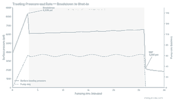
P_surface = 7,347 − 3,731 + 4,722 = 8,338 psi — that’s the number to expect on the gauge at the moment of breakdown, and it’s a long way from the 7,347 psi bottomhole figure. Skip the friction term and you’ll misjudge breakdown by nearly 60%.

Step 4: Pump to breakdown and record the ISIP

In the field, you don’t need to hit the predicted number exactly — you need to recognize it. The signature is a sharp pressure peak followed by an immediate fall as the fracture opens and takes fluid faster than friction can resist it. Once the main treatment stage finishes, the pumps shut down and the surface pressure drops almost instantly to the instantaneous shut-in pressure (ISIP) — the pressure the instant friction disappears but before the fracture has had time to close.

Step 5: Convert surface ISIP to bottomhole ISIP

Once the pumps are off, friction is gone — the only correction left is hydrostatic, using the density of whatever fluid actually fills the wellbore at that moment (proppant-laden slurry is denser than the clean pad fluid you started with):

BH-ISIP = Surface ISIP + ρ_slurry×TVD/144

At SG 1.15, the slurry hydrostatic gradient is 0.498 psi/ft, or 4,086 psi over 8,200 ft. BH-ISIP = 2,150 + 4,086 = 6,236 psi.

Step 6: Calculate net pressure and read the trend

Net pressure is what’s left once you subtract the rock’s resistance to opening — the closure pressure, σ_h,min — from the bottomhole pressure actually achieved:

P_net = BH-ISIP − σ_h,min = 6,236 − 5,740 = 496 psi

A positive net pressure in the 200–1,000 psi range, like this one, is the signature of a fracture propagating with reasonably contained height growth. Watch the trend across a treatment, not just one value: net pressure climbing stage over stage usually means the fracture is running out of room (approaching a barrier or depleting nearby); flat net pressure suggests steady, unconfined propagation; and a sudden net pressure spike mid-stage, together with a rate drop, is the classic screenout signature — proppant bridging faster than fluid can carry it away.

Step 7: Automate it in Python

The hand calculation above is worth doing once per field area to build intuition for the numbers. For live monitoring, you want the ISIP and net pressure pulled automatically out of the pressure-and-rate time series every stage records. A simple rule works well: ISIP is the pressure at the first sample where rate has fallen to zero after having been above a pumping threshold.

import pandas as pd

def breakdown_pressure(sigma_h_min, sigma_H_max, pore_p, tensile_strength):
    """Hubbert & Willis bottomhole breakdown pressure, vertical well."""
    return 3 * sigma_h_min - sigma_H_max - pore_p + tensile_strength

def find_isip(df, time_col="time_min", rate_col="rate_bpm", press_col="pressure_psi",
              pump_threshold=5.0):
    """df must be sorted by time. Returns (isip_time, isip_pressure)."""
    was_pumping = df[rate_col] > pump_threshold
    shut_in = was_pumping.shift(1, fill_value=False) & (df[rate_col] <= pump_threshold)
    idx = df.index[shut_in]
    if len(idx) == 0:
        raise ValueError("No shut-in detected: rate never drops below threshold")
    first = idx[0]
    return df.loc[first, time_col], df.loc[first, press_col]

def net_pressure(surface_isip, tvd_ft, slurry_sg, closure_pressure_psi):
    bh_isip = surface_isip + slurry_sg * 62.4 * tvd_ft / 144.0
    return bh_isip - closure_pressure_psi, bh_isip

# Pre-job prediction
Pbd = breakdown_pressure(5740, 6560, 3813, 500)
print(f"Bottomhole breakdown pressure: {Pbd:.0f} psi")   # 7347 psi

# After the job: df loaded from the frac van's pressure/rate log
# t, isip = find_isip(df)
isip_surface = 2150.0
pnet, bh_isip = net_pressure(isip_surface, 8200, 1.15, 5740)
print(f"Bottomhole ISIP: {bh_isip:.0f} psi, net pressure: {pnet:.0f} psi")
# Bottomhole ISIP: 6236 psi, net pressure: 496 psi

Run find_isip on every stage in a well's job log with pandas, store the net pressure trend alongside stage number, and you get a stage-by-stage containment diagnostic without anyone staring at a live screen trying to eyeball a spike. Pair it with the proppant side of the job using our proppant settling velocity calculation, and with a broader look at the diagnostic software landscape in Best AI Tools for Hydraulic Fracturing Diagnostics.

How to verify it worked

1. Breakdown exceeds closure: P_bd (bottomhole) must always be greater than σ_h,min — here 7,347 > 5,740 — or the stress inputs are inconsistent.
2. ISIP sits below the breakdown peak: BH-ISIP (6,236 psi) should be noticeably lower than the bottomhole breakdown pressure (7,347 psi); once the fracture exists, propagating it takes less pressure than creating it did.
3. Net pressure is plausible: for a contained, propagating fracture, expect roughly 200–1,000 psi. A calculated net pressure near zero or negative usually means the closure pressure estimate is too high, not that the fracture failed to open.

Common pitfalls

• Mistaking a water-hammer transient for the true ISIP. The instant pumps stop, a pressure oscillation can ring through the fluid column for a few seconds; read ISIP after it settles, not at the first local peak or trough.
• Using the wrong fluid density for the hydrostatic correction. Clean pad fluid, cross-linked gel, and proppant-laden slurry all have different densities — use the density of whatever is actually in the wellbore at the specific moment you're correcting, not the density you started the stage with.
• Treating closure pressure as a fixed input. σ_h,min from an old offset test can drift from reality after prior stages have already altered near-wellbore stress; a step-down test on the current well beats a borrowed number whenever one is available.

Breakdown pressure answers a question you need before the job starts; net pressure answers one you need while it's running. Calculate both in advance, build the ISIP-extraction script once, and the live pressure chart stops being something you read on instinct and starts being a number you can actually trust.