
By Saad Iqbal
The wireline unit is still on location, the mud engineer wants a number before anyone changes the program, and the only fresh data in the room is a resistivity curve that just rolled over. Nobody wants to wait three days for a full pore pressure study when the well is three hundred feet from a casing point. This is exactly the situation Ben Eaton’s 1975 method was built for: turn a single resistivity departure from the normal compaction trend into a defensible pore pressure gradient, by hand, in about the time it takes to read this sentence twice. Once you’ve done it once with a calculator, it’s eight lines of Python you never do by hand again.
Why Eaton’s Method Still Runs the Well-Site Laptop
Modern basin-modelling software will give you a beautifully smoothed pore pressure profile from seismic velocities, offset-well calibration and a geomechanical earth model. None of that helps the mudlogger at 2 a.m. when the resistivity tool just logged through a shale interval that’s clearly diverging from everything above it. Eaton’s resistivity method survives because it needs nothing more than a normal compaction trend line and the resistivity reading in front of you, and it’s the same equation every pore-pressure-while-drilling service runs under the hood. Knowing how to run it yourself means you can sanity-check the vendor’s number instead of just trusting the screen.
Prerequisites
- A resistivity log (deep reading, shale-corrected) over the interval of interest
- A normal compaction trend line fit through shale resistivity in normally pressured sections above
- Overburden gradient (OBG), from a density log integration or a regional estimate
- Normal hydrostatic pressure gradient (Pn) for the mud/formation water system, typically 0.433–0.465 psi/ft
- True vertical depth of the point you’re evaluating
- Python 3 with pandas installed, if you want to run the automation step
Step 1 — Establish the Overburden and Normal Pressure Trends
Eaton’s equation measures pore pressure as a departure between two straight lines: the overburden gradient (the ceiling, from the weight of everything above) and the normal hydrostatic gradient (the floor, if pressure were behaving normally). For this tutorial’s worked well, OBG = 1.00 psi/ft — a reasonable regional average once you’re a few thousand feet below the mudline — and Pn = 0.465 psi/ft, matching a moderately saline formation water system. Why it matters: every pore pressure number Eaton’s method produces sits somewhere between these two lines, so getting them right first is what keeps the final answer physically sane rather than just mathematically tidy.

Step 2 — Read the Resistivity Departure from the Normal Trend
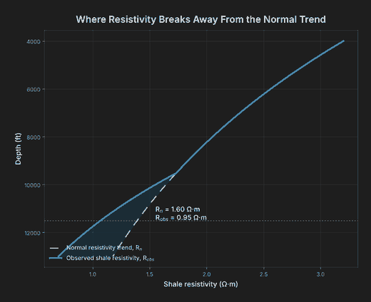
In a normally compacting shale, resistivity rises steadily with depth as the rock compacts and loses porosity — plot that trend on a log scale and it’s close to a straight line. Overpressure shows up as a shale that’s more porous, and therefore less resistive, than its depth alone would predict: the observed curve sags below the normal trend. Draw your normal trend line through clean shale points in the normally pressured section above, then read two numbers at your depth of interest: Rn, the resistivity the normal trend line predicts at that depth, and Robs, what the log actually reads. For this well at 11,500 ft TVD: Rn = 1.60 Ω·m, Robs = 0.95 Ω·m — a clear downward departure, and departure is the entire signal Eaton’s method runs on.
Step 3 — Apply Eaton’s Equation
With both trend lines and the resistivity departure in hand, Eaton’s resistivity equation converts the ratio directly into a pore pressure gradient:
PP = OBG − (OBG − Pn) × (Robs / Rn)^n

PP   = pore pressure gradient, psi/ft
OBG  = overburden gradient, psi/ft
Pn   = normal hydrostatic pressure gradient, psi/ft
Robs = observed resistivity at depth, Ω·m
Rn   = normal trend resistivity at depth, Ω·m
n    = Eaton exponent, commonly 1.2 for resistivity (1.0–1.5 range by basin)
Plugging in the worked numbers — OBG = 1.00 psi/ft, Pn = 0.465 psi/ft, Robs = 0.95 Ω·m, Rn = 1.60 Ω·m, n = 1.2:
Robs / Rn = 0.95 / 1.60 = 0.594
0.594^1.2 = 0.535

PP = 1.00 − (1.00 − 0.465) × 0.535
   = 1.00 − 0.535 × 0.535
   = 1.00 − 0.286
   = 0.714 psi/ft

Pore pressure at 11,500 ft = 0.714 × 11,500 ≈ 8,209 psi
That 0.714 psi/ft gradient sits well above the 0.465 psi/ft normal line and still comfortably under the 1.00 psi/ft overburden ceiling — exactly the moderate-to-significant overpressure signature a resistivity sag like this one should produce.

Step 4 — Convert the Gradient to Equivalent Mud Weight
A psi/ft gradient is correct but not what anyone on the rig floor thinks in. Convert it to equivalent mud weight (EMW) in ppg, the number that actually gets compared against the mud weight in the hole, using the standard oilfield constant:
EMW (ppg) = Pore Pressure Gradient (psi/ft) / 0.052

EMW = 0.714 / 0.052 = 13.73 ppg
13.73 ppg is the floor of your mud weight window at 11,500 ft on this well — drop below it and you’re inviting a kick. Compare that number against your fracture gradient (see our MAASP calculation guide for the companion ceiling-side math) before you finalize the mud program.

Step 5 — Automate It With Python and pandas
One depth point is a useful sanity check; a whole well log is where automation earns its keep. Python with pandas turns the same equation into something you run once per well instead of once per depth point:
import pandas as pd

def eaton_pp_gradient(obg_psift, pn_psift, robs_ohmm, rn_ohmm, n=1.2):
    """Eaton's resistivity method: pore pressure gradient, psi/ft."""
    ratio = robs_ohmm / rn_ohmm
    return obg_psift - (obg_psift - pn_psift) * (ratio ** n)

df = pd.DataFrame({
    "depth_ft":  [10000, 10500, 11000, 11500],
    "obg_psift": [1.00,  1.00,  1.00,  1.00],
    "pn_psift":  [0.465, 0.465, 0.465, 0.465],
    "rn_ohmm":   [1.80,  1.72,  1.66,  1.60],
    "robs_ohmm": [1.75,  1.40,  1.10,  0.95],
})

df["pp_gradient_psift"] = eaton_pp_gradient(
    df.obg_psift, df.pn_psift, df.robs_ohmm, df.rn_ohmm
)
df["pp_psi"]   = df.pp_gradient_psift * df.depth_ft
df["emw_ppg"]  = df.pp_gradient_psift / 0.052

print(df[["depth_ft", "pp_gradient_psift", "pp_psi", "emw_ppg"]].round(3))
#    depth_ft  pp_gradient_psift   pp_psi  emw_ppg
# 0     10000              0.496   4960.0    9.538
# 1     10500              0.560   5880.0   10.769
# 2     11000              0.636   6996.0   12.231
# 3     11500              0.714   8211.0   13.731
Notice the last row matches the hand calculation from Step 3 almost exactly — the tiny difference is only rounding. Swap the four input columns for your own LAS-derived resistivity and trend-line values and the whole log recalculates in a fraction of a second, every time a new section is logged.

Expected Result and How to Verify It
For this well at 11,500 ft TVD, you should land on a pore pressure gradient of 0.714 psi/ft, a pore pressure of roughly 8,209 psi, and an equivalent mud weight of 13.73 ppg. Verify it two ways before trusting it on a live well: first, confirm the result sits strictly between Pn and OBG — if your answer comes out above the overburden gradient or below normal hydrostatic, you’ve made an arithmetic or sign error, not found real pressure. Second, run the same inputs through the Python function and the hand calculation separately and confirm they agree to within rounding; a large mismatch almost always means a units slip, not a bad formula.
Common Pitfalls
- Fitting the normal trend line through compacting, not normally pressured, shale. If the “normal” section you calibrate against is itself mildly overpressured, every Rn you read off it is too low, and the whole log underpredicts pore pressure below it.
- Using a borrowed Eaton exponent without checking it against a known pressure point. n = 1.2 is a common resistivity default, but basins vary from roughly 1.0 to 1.5 — calibrate against an offset well’s measured pressure (an RFT/MDT point or a kick) wherever you have one, rather than trusting a textbook value blind.
- Forgetting shale-bed correction. Resistivity picked from a thin sand or a washed-out interval isn’t shale resistivity at all — always confirm you’re reading clean, shale-only points on both the normal trend and the observed curve.
Once pore pressure is locked down, the natural next check is the fracture gradient ceiling above it — our MAASP calculation guide walks through that companion well-control math, and if you’re also tracking trip-speed margins against this same pore pressure line, see our surge and swab pressure tutorial. For a broader look at how geomechanics platforms handle this at scale, our roundup of AI wellbore stability tools is worth reading next.
Got a resistivity log with a departure you’re not sure how to read? Run the numbers through the script above before your next casing-point decision and see where it lands relative to your mud weight.
