
By Saad Iqbal
The weight indicator stops climbing. You keep pumping the reel forward, but the depth counter has frozen at 8,240 ft, and the only thing increasing is surface pressure. Somewhere downhole, the coiled tubing has stopped transmitting force to the bottom and started helically coiling against the inside of the production tubing instead — a lockup. If you had run the coiled tubing lockup prediction numbers before the job, you would have known the string was going to buckle a few hundred feet short of target, and you could have picked a lighter string, a slicker fluid, or a different deployment method before ever picking up the reel. This tutorial walks through exactly how to calculate that buckling and lockup force by hand and in Python, using the same Dawson-Paslay mechanics that service company tubing-forces software runs under the hood.
What you need before you calculate coiled tubing buckling
PREREQUISITES — have these on hand before you start:
- CT outside diameter (OD) and inside diameter (ID), or OD and nominal wall thickness, for the reel you’re running
- CT weight per foot in air, from the mill certificate or tubing-forces reference table
- Working fluid density (and whether you’re also pumping nitrogen — if so, see our nitrogen volume calculation for CT N2 jobs first)
- Radial clearance between the CT OD and the ID of the tubing or casing it’s running inside
- A deviation survey for the well, or at minimum the inclination at the critical depth you’re worried about
- Young’s modulus for the CT material grade (30×10⁶ psi for standard carbon steel CT)
- A Python environment, or a spreadsheet, to run the calculation
With those seven inputs in hand, the buckling calculation itself is six short steps.
Step 1 — Get the pipe’s cross-sectional properties
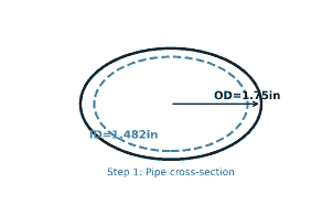
What to do: From the OD and ID, calculate the moment of inertia, I. For a common 1.75 in OD CT string with a 1.482 in ID (0.134 in nominal wall), use the standard tube formula:
I = (π / 64) × (OD⁴ − ID⁴)
Why it matters: Every buckling equation downstream is driven by I. A thinner-wall CT string (lower I) buckles at a dramatically lower force than a heavier-wall string of the same OD — this is the single biggest lever you have when a lockup prediction comes back unfavorable.
Worked example: OD = 1.75 in, ID = 1.482 in.
OD⁴ = 9.3789, ID⁴ = 4.8238
I = (π/64) × (9.3789 − 4.8238) = 0.2237 in⁴
Step 2 — Compute the buoyed weight in your working fluid
What to do: Buckling force depends on the pipe’s weight in the fluid it’s running in, not its weight in air. Apply a buoyancy factor to the air weight:
BF = 1 − (ρ_fluid / 65.4), with ρ_fluid in ppg
Why it matters: Buoyancy is free lockup protection. Running CT in an 8.5 ppg brine instead of displacing it to a heavier kill-weight fluid can shave 10-15% off the effective weight driving the string into compression against friction — directly pushing the lockup depth deeper.
Worked example: Air weight = 2.31 lbf/ft. In 8.5 ppg brine, BF = 1 − (8.5/65.4) = 0.870.
Buoyed weight = 2.31 × 0.870 = 2.01 lbf/ft.

Step 3 — Determine the radial clearance
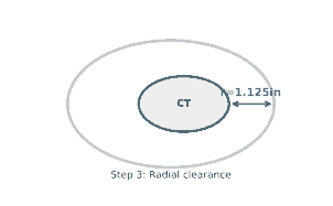
What to do: Radial clearance, r, is half the difference between the ID of whatever the CT is running inside (production tubing, liner, or open hole) and the CT’s own OD:
r = (ID_tubing − OD_CT) / 2
Why it matters: Clearance and buckling force are inversely related — tighter clearance buckles sooner. This is why lockup problems appear almost exclusively inside small-ID production tubing or liner, not in open hole or large-ID casing, and why a seemingly minor tubing size change between wells can turn a routine job into a lockup.
Worked example: For CT running inside 3.5 in, 9.3 lb/ft tubing (ID ≈ 3.0 in) against a 1.75 in OD string: r = (3.0 − 1.75)/2 ≈ 1.125 in once ovality and connector OD are accounted for — use the manufacturer’s clearance table for your exact tubing/CT pairing rather than a raw ID subtraction.
Step 4 — Calculate the critical sinusoidal and helical buckling forces
What to do: Use the Dawson-Paslay critical sinusoidal buckling force, then the helical (lockup) threshold:
Fcr,sin = √(8 × E × I × w × sinθ / r)Fcr,hel = √2 × Fcr,sin
Why it matters: Sinusoidal buckling (the pipe snaking side-to-side against the wall) is a warning sign — friction jumps, but the string can usually still advance. Helical buckling (the pipe corkscrewing) is where lockup happens: once axial compressive force exceeds Fcr,hel, additional surface push stops converting to downhole reach at all.
Worked example, at a 45° inclination in the curve section (E = 30×10⁶ psi, I = 0.2237 in⁴, w = 2.01 lbf/ft, r = 1.125 in, sin 45° = 0.7071):
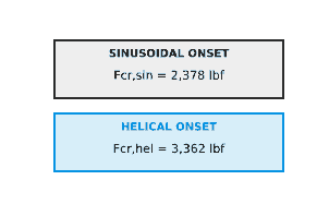
Fcr,sin = √(8 × 30,000,000 × 0.2237 × (2.01/12) × 0.7071 / 1.125) ≈ 2,378 lbf
Fcr,hel = √2 × 2,378 ≈ 3,362 lbf
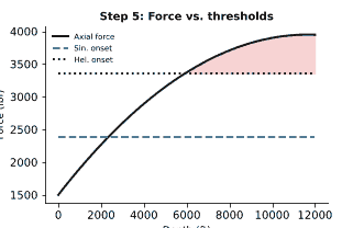
Step 5 — Plot the actual force profile against the thresholds
What to do: The two numbers from Step 4 are thresholds, not a prediction by themselves. Build (or pull from your tubing-forces software) the actual axial compressive force at the bottom of the string as a function of depth — driven by the CT’s own buoyed weight below the point in question plus accumulated friction drag, which you can estimate with our coiled tubing friction pressure calculation — then overlay it on Fcr,sin and Fcr,hel.
Why it matters: This is the step that actually answers “will I lock up, and at what depth?” The force curve crossing Fcr,sin tells you where friction starts climbing; crossing Fcr,hel tells you where the job stops making hole. Everything upstream of this step just builds the two threshold lines.
Worked example: On a typical curve-to-horizontal CT intervention, cumulative friction plus buoyed string weight can push the compressive end-load past 3,362 lbf well before target depth — exactly the kind of lockup risk zone shown shaded in the chart below. Once your curve crosses into that zone, no amount of extra surface force helps; you need to change the plan, not push harder.
Step 6 — Know the pitfalls that throw off a lockup prediction
What to do: Before you trust the number, check for these four common sources of error:
- Using air weight instead of buoyed weight — this alone can overstate buckling risk by 10-15%
- Using nominal clearance instead of the connector OD and actual tubing drift, which is almost always the tighter constraint
- Ignoring friction factor uncertainty — a friction factor that’s off by 0.05 can move the predicted lockup depth by hundreds of feet
- Treating buckling as binary rather than checking the full force-vs-depth curve at every significant inclination change, since lockup risk is highest right where the wellbore curves fastest
Why it matters: A lockup prediction is only as good as its weakest input. Most “the software said we’d reach bottom” surprises trace back to one of these four shortcuts, not to the buckling formula itself.

Automate it in Python
Here is the full Step 1-4 calculation as a reusable Python function, so you can run it for every reel size and well profile in your program without rebuilding the spreadsheet each time:
import math

def ct_buckling_thresholds(OD, ID, E, w_air, fluid_ppg, r, theta_deg):
    """
    Returns (I, w_buoyed, Fcr_sin, Fcr_hel) for a coiled tubing
    lockup-prediction check.

    OD, ID      : coiled tubing outside/inside diameter, inches
    E           : Young's modulus, psi (30e6 for carbon steel CT)
    w_air       : CT weight in air, lbf/ft
    fluid_ppg   : working fluid density, ppg
    r           : radial clearance, inches
    theta_deg   : wellbore inclination at the point checked, degrees
    """
    I = (math.pi / 64) * (OD**4 - ID**4)              # in^4
    BF = 1 - (fluid_ppg / 65.4)                         # buoyancy factor
    w_buoyed = w_air * BF                               # lbf/ft
    w_per_in = w_buoyed / 12.0                          # lbf/in
    sin_theta = math.sin(math.radians(theta_deg))

    Fcr_sin = math.sqrt(8 * E * I * w_per_in * sin_theta / r)
    Fcr_hel = math.sqrt(2) * Fcr_sin
    return I, w_buoyed, Fcr_sin, Fcr_hel


I, w_buoyed, Fcr_sin, Fcr_hel = ct_buckling_thresholds(
    OD=1.75, ID=1.482, E=30e6, w_air=2.31,
    fluid_ppg=8.5, r=1.125, theta_deg=45.0,
)

print(f"I          = {I:.4f} in^4")
print(f"w_buoyed   = {w_buoyed:.2f} lbf/ft")
print(f"Fcr,sin    = {Fcr_sin:,.0f} lbf")
print(f"Fcr,hel    = {Fcr_hel:,.0f} lbf")
Loop that function over your deviation survey’s inclination at each 100 ft interval, compare against your friction-drag-plus-weight force profile, and you have a full lockup-depth prediction without opening a commercial tubing-forces license — useful for a quick first pass before committing to the full model. For the inclination-dependent geometry inputs, NumPy array operations let you vectorize the whole survey in a few lines instead of looping row by row.
What a good result looks like — and how to verify it
A trustworthy lockup prediction gives you a specific depth or inclination range where the force curve crosses Fcr,hel, not just a pass/fail on the whole run. Verify it two ways before you commit to a plan: first, sanity-check Fcr,sin against a published worked example for similar CT and clearance (PetroWiki’s buckling reference example is a good cross-check); second, re-run the calculation with your buoyed weight deliberately swapped back to air weight — if the lockup depth moves by more than a few hundred feet, you know how sensitive your result is to that one input, which tells you how carefully to pin it down before the job. If your actual force profile stays comfortably below Fcr,sin across the whole planned interval, you’re not just avoiding lockup — you’re avoiding the friction penalty that sinusoidal buckling adds on the way there.
Buckling mechanics on a CT string follow the same beam-column physics as a conventional drill string — if you’re planning a directional well with a jointed string instead, our torque and drag calculation using the soft-string model walks through the equivalent force-and-friction buildup for that case.
