Torque & Drag Calculation: The Soft-String Model

By Saad Iqbal

Picture a directional driller watching the weight indicator during a trip, trying to decide whether the string is hanging up on a tight dogleg or simply carrying the friction a 45-degree build section always carries. Guess wrong and you either rip into a ledge or waste a shift pulling out “just to be safe.” A proper torque and drag calculation using the soft-string model turns that guess into a number: it predicts the hookload you should see at surface, before you ever pick up the pipe. This tutorial walks through the governing equations, a full worked numeric example on a build-and-hold well, and verified Python code you can reuse on your own survey data.

What You’ll Need Before You Start

Prerequisites

A directional survey: measured depth (MD) and inclination at each station, at minimum.
Drill string data: pipe OD, weight per foot in air, and mud weight (to compute the buoyancy factor).
An assumed sliding friction factor between pipe and wellbore — 0.2–0.35 is typical, higher in open hole than cased hole.
Python 3.9+ (free from python.org); no third-party library is strictly required, though NumPy makes the arithmetic cleaner.

If your survey still needs to be turned into MD/inclination/azimuth stations from raw tool readings, start with Minimum Curvature Method: Automate Directional Drilling Surveys — everything below assumes that step is already done.

Step 1: Lay Out the Wellbore Trajectory

The soft-string model — first published by Johancsik, Friesen, and Dawson in 1984 (SPE-11380-PA) — treats the drill string as a flexible cable lying along the wellbore, with no bending stiffness of its own. That simplification is exactly why it’s still the default first pass: it needs nothing more than the survey stations and basic pipe data to run. For this example we’ll use a simple build-and-hold well:

Vertical section: 0–3,000 ft MD, inclination 0° throughout.
Build section: 3,000–4,500 ft MD, inclination builds from 0° to 45° (a 3°/100 ft build rate).
Tangent section: 4,500–8,000 ft MD, holding at 45° to total depth.

Why it matters: every segment where inclination is changing (the build section) generates extra normal force beyond simple gravity, because the pipe is being forced to curve against the wellbore wall. That’s the piece a flat, no-friction weight calculation always misses.

Step 2: Draw the Free Body and Define the Governing Equations

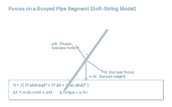
Look at any short segment of pipe in the hole and three things act on it: its own buoyed weight, a normal (contact) force from the wellbore wall, and a friction force along the pipe that opposes whatever direction it’s sliding. The soft-string model turns that free body into three equations, applied segment by segment up the wellbore:

Normal force: F_N = √[ (w · ΔL · sinθ_avg)² + (T · Δθ)² ]

Incremental tension: ΔT = w · ΔL · cosθ_avg ∓ μ · F_N (− while lowering, + while hoisting)

Incremental torque: ΔM = μ · F_N · r

where w is buoyed weight per foot (lbf/ft), ΔL is the segment length (ft), θ_avg is the average inclination over the segment, Δθ is the change in inclination across the segment (radians), T is the tension already carried into the segment (lbf), μ is the sliding friction factor, and r is the pipe radius (ft). Why the sign flips between lowering and hoisting: friction always opposes the direction of motion, so when you’re running pipe in, friction acts upward and reduces the tension buildup; when you’re pulling out, friction acts downward and adds to it — which is exactly why pick-up weight always reads higher than slack-off weight on a real rig.

Step 3: Work the Arithmetic for One Segment

Take 5-inch drill pipe at 19.5 lbf/ft in air, running in 10 ppg mud (buoyancy factor ≈ 0.85, so buoyed weight w = 19.5 × 0.85 = 16.6 lbf/ft), with a sliding friction factor μ = 0.25. Start at the bit (T = 0, no weight on bit) and work the build section first, since it carries tension already accumulated from the tangent section below it. By the time the string reaches the top of the tangent section, tension is 30,812 lbf. Through the 1,500 ft build section (ΔL = 1,500 ft, θ_avg = 22.5°, Δθ = 45° = 0.7854 rad):

F_N = √[ (16.6 × 1500 × sin22.5°)² + (30,812 × 0.7854)² ] = √[ 9,520² + 24,196² ] ≈ 26,008 lbf

ΔT (lowering) = 16.6 × 1500 × cos22.5° − 0.25 × 26,008 = 22,995 − 6,502 ≈ 16,503 lbf

So tension at the top of the build section is 30,812 + 16,503 = 47,315 lbf. Notice the curvature term (24,196) is actually larger than the pure-gravity term (9,520) in this segment — that’s the build section’s dogleg doing exactly what the flat calculation would have missed entirely.

Step 4: Automate the Full Wellbore in Python

Doing one segment by hand builds intuition; doing all of them by hand on a real multi-station survey is how NPT happens. The function below walks every segment from bit to surface and returns the full tension and torque profile, for either lowering or hoisting.

import math

def soft_string_profile(segments, w, mu, r, mode="lower"):
    """
    segments: list of (name, md_deep, md_shallow, inc_deep_deg, inc_shallow_deg),
              ordered from the bit upward to surface.
    w   : buoyed weight per unit length, lbf/ft
    mu  : sliding friction factor
    r   : pipe radius, ft
    mode: "lower" (running in) or "hoist" (pulling out)
    Returns a list of per-segment results and the total surface torque.
    """
    T = 0.0
    total_torque = 0.0
    profile = []
    for name, md_deep, md_shallow, inc_deep, inc_shallow in segments:
        dL = md_deep - md_shallow
        theta_avg = math.radians((inc_deep + inc_shallow) / 2.0)
        dtheta = math.radians(abs(inc_deep - inc_shallow))

        F_N = math.sqrt((w * dL * math.sin(theta_avg)) ** 2 + (T * dtheta) ** 2)
        sign = -1.0 if mode == "lower" else 1.0
        dT = w * dL * math.cos(theta_avg) + sign * mu * F_N
        dM = mu * F_N * r

        T += dT
        total_torque += dM
        profile.append({"segment": name, "F_N_lbf": F_N, "dT_lbf": dT,
                         "T_end_lbf": T, "dM_ftlbf": dM})
    return profile, T, total_torque

segments = [
    ("Tangent",  8000, 4500, 45.0, 45.0),
    ("Build",    4500, 3000, 45.0,  0.0),
    ("Vertical", 3000,    0,  0.0,  0.0),
]

profile, T_surface, M_surface = soft_string_profile(
    segments, w=16.6, mu=0.25, r=2.5 / 12.0, mode="lower"
)
for seg in profile:
    print(f"{seg['segment']:9s}  F_N={seg['F_N_lbf']:9,.0f} lbf  "
          f"dT={seg['dT_lbf']:9,.0f} lbf  T_end={seg['T_end_lbf']:10,.0f} lbf")
print(f"Surface hookload (slack-off): {T_surface:,.0f} lbf")
print(f"Surface torque (rotating):    {M_surface:,.0f} ft-lbf")

Why walk from the bit upward rather than from surface down: tension at any point depends on everything hanging below it, so you need the deepest point’s tension (zero, with no weight on bit) before you can work out the next segment up. Get the direction of integration backward and every number downstream of that mistake is wrong, even though the code runs without a single error.

Step 5: Read the Output and Compare Lowering vs. Hoisting

Run the function once with mode="lower" and once with mode="hoist" and put the two surface numbers side by side against the frictionless (straight-line) weight. For this well, the frictionless hanging weight is 113,888 lbf. The soft-string model predicts:

Slack-off (lowering): 97,115 lbf — friction is helping support roughly 16,800 lbf of string weight.
Pick-up (hoisting): 134,519 lbf — friction now resists the pull, adding roughly 20,600 lbf.

That 37,400 lbf spread between pick-up and slack-off weight, straddling the frictionless value, is the signature pattern you should see on every trip sheet — if your real rig data doesn’t straddle the frictionless weight in roughly that shape, your assumed friction factor is off and worth revisiting against AI torque and drag optimization tools that calibrate friction factor automatically from real-time data.

What Result Should You Expect?

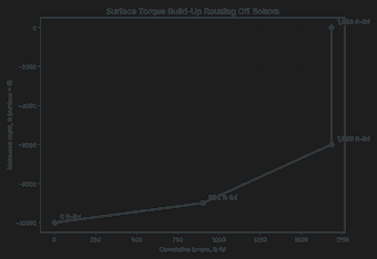
For this build-and-hold well, expect a slack-off hookload around 97,000 lbf, a pick-up weight around 134,500 lbf, and a rotating torque near 3,500 ft-lbf. The exact numbers will shift with your friction factor, mud weight, and survey — but the pattern (pick-up > frictionless > slack-off, with torque concentrated in the curved sections) should hold on every well.

Sanity Check Your Answer

Set μ = 0 in the code and confirm you recover the frictionless hanging weight exactly — that isolates whether your trajectory and weight inputs are right before friction is even in the picture. Then confirm slack-off < frictionless < pick-up; if that ordering is reversed, your sign convention on ΔT is flipped.

Common Pitfalls

Ignoring the curvature term in build and turn sections. As Step 3 showed, it can dominate the normal force — dropping it understates friction everywhere torque and drag actually matter most.
Using one friction factor for the whole well. Cased hole and open hole, and water- versus oil-based mud, can easily differ by 0.1 or more; a single blended value hides where the real drag is coming from.
Forgetting the soft-string model has no bending stiffness. In tight-radius doglegs or highly deviated short-radius wells, a stiff-string model will predict meaningfully different, usually higher, contact forces — treat soft-string results as a reasonable first pass, not the final word on a tricky well.

For a dedicated library rather than hand-rolled functions, Pro Well Plan’s open-source torque-drag package runs the same soft-string physics across a full survey with one function call, and it’s worth cross-checking against if you’re putting this into a production workflow. And if torsional vibration rather than drag is what’s keeping you up at night, AI Stick-Slip Detection covers the real-time surface-torque signature that follows naturally from the torque equation above.