

By Saad Iqbal
A production choke that worked perfectly for eighteen months can fail in an afternoon once sand starts moving with the fluid. There’s no dramatic warning, no spike that trips an obvious alarm — just a slow, quiet thinning of metal at the one bend the flow stream hits hardest, until one day it doesn’t hold. AI erosion monitoring exists because that failure mode is almost entirely preventable, if you’re tracking the right number continuously instead of discovering it during a shutdown inspection.
The Number That Actually Matters: Erosional Velocity
API RP 14E defines a practical erosional velocity limit for sizing piping and fittings in erosive service:
Ve = C / √ρm
where Ve is the erosional velocity limit in ft/s, ρm is the mixture density in lb/ft³, and C is an empirical constant tied to how erosive the service is. Take a gas-condensate stream with a mixture density of 20 lb/ft³ running in continuous service, where API RP 14E suggests C = 100:
Ve = 100 / √20 = 100 / 4.47 = 22.4 ft/s
Cross that line regularly and you’re not failing tomorrow, but you’re drawing down the wall thickness on borrowed time. The table below shows how the C-factor itself changes the picture, which is exactly why a single static limit baked into a P&ID years ago stops being useful once the well starts making sand.
| Service Type | Typical C-Factor | Ve at ρm = 20 lb/ft³ |
|---|---|---|
| Continuous service, solids present | 100 | 22.4 ft/s |
| Noncontinuous / intermittent service | 125 | 28.0 ft/s |
| Solids-free, corrosion-inhibited, non-corrosive fluids | 150–200 | 33.5–44.7 ft/s |
That spread matters in practice. Field studies on gas-condensate wells have shown that operators applying a higher, better-justified C-value — rather than defaulting to the conservative 100 — can run meaningfully higher rates without exceeding a realistic erosion risk, provided they’re actually monitoring wall loss rather than assuming the conservative number protects them forever.
Where Erosion Actually Concentrates
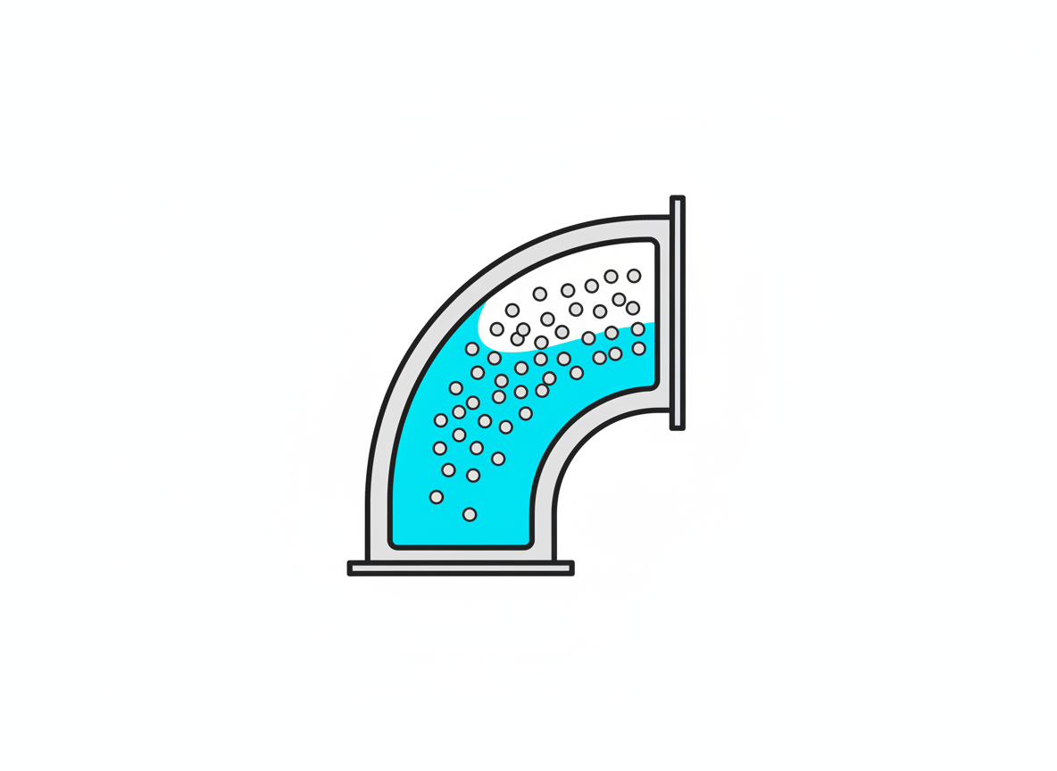
Erosion isn’t evenly distributed along a flowline. Sand particles carry momentum in a straight line; it’s the outer wall of every elbow, the body of every choke, and the downstream face of every tee that takes the direct impact. A straight run of pipe can run for years with negligible wall loss while the elbow fifty feet downstream is already thinning. That’s why a single wellhead-pressure-based production limit misses the real risk: it treats the whole flow path as uniform when the damage is concentrated in a handful of predictable geometric hotspots.
How Does AI Erosion Monitoring Actually Work?
Non-intrusive acoustic sand and erosion monitors clamp onto the outside of the pipe at those known hotspots and listen for the high-frequency signature of particle impacts against the wall, converting that signal into a real-time sand production rate and a cumulative erosion estimate. A thickness-sensing probe, by contrast, measures actual remaining wall thickness directly, trading some installation complexity for a ground-truth number. The genuinely new piece isn’t either sensor — both have existed for years — it’s the layer that fuses readings from several hotspots with the current flow rate, choke position, and fluid composition to flag a trend before it crosses a hard limit, rather than waiting for a single sensor to breach its own threshold. That’s a meaningfully different alarm philosophy: instead of “this point just failed its check,” it’s “this point’s erosion rate has accelerated 3x over two weeks and will cross its wall-loss limit in nine days at the current production rate.”
Vendors like Emerson, through its Roxar corrosion and erosion monitoring line, combine acoustic sand detection with corrosion probes on the same monitoring backbone, which matters because sand erosion and internal corrosion often accelerate each other: erosion strips away a pipe’s protective scale, and the freshly exposed metal corrodes faster, which in turn roughens the surface and increases local turbulence and erosion. Treating the two as separate problems monitored by separate systems misses that feedback loop.
Sizing a Monitoring Program: Where to Put Sensors First
Most operators can’t instrument every elbow and choke on every well, so the sensor budget has to go where the physics says the risk concentrates first. Start with the production choke itself: it sees the highest velocity and the sharpest pressure drop on the entire flowline, which is exactly the combination that accelerates erosion fastest. Next come the first two or three elbows downstream of the choke, before the velocity has a chance to settle back into a straight run. A well with a known or suspected sand production trend — rising with increasing drawdown, or a step change after a workover — deserves monitoring before first oil, not after a first failure prompts a retrofit. For wells without a strong sand signal yet, a lighter instrumentation plan at the choke alone, with periodic ultrasonic thickness surveys at the downstream elbows, is a reasonable starting budget that can be expanded once the data justifies it. The mistake to avoid is treating the monitoring plan as fixed: a well that starts clean often doesn’t stay that way as reservoir pressure depletes and drawdown increases to compensate.
Reading the Trend, Not Just the Threshold
The practical shift AI brings is less about detecting a single event and more about separating normal production noise from a genuine wear trend. Acoustic sand signals are noisy — a choke adjustment, a slug of liquid, or a transient flow surge can all spike the raw signal without indicating sustained erosion. A model trained on months of a well’s own baseline behavior can tell the difference between a five-minute transient and a trend that’s been climbing steadily for two weeks, which is exactly the distinction a simple fixed-threshold alarm can’t make. That lets engineers set a production choke position based on actual, current erosion risk instead of a conservative number chosen on day one of first oil and never revisited.
Where Engineers Should Stay Skeptical
- Acoustic monitors infer, they don’t measure wall thickness directly. Calibrate acoustic sand-rate estimates against periodic ultrasonic thickness surveys, don’t trust the acoustic number alone for long-term wall-loss tracking.
- C-factor selection is a judgment call, not a lookup. Pushing toward the 150–200 range without solids-free, non-corrosive conditions genuinely present is how a conservative guideline turns into a real failure.
- Sensor placement decides what you actually catch. A monitor on the wrong elbow tells you nothing about the one that’s actually thinning.
- Flow regime changes shift the hotspots. A well transitioning from low to high water cut, or changing choke size significantly, can relocate where erosion concentrates — monitoring plans built at first oil need revisiting as the well matures.
For engineers building their own trending layer on top of raw sensor exports, a Python and pandas pipeline that computes a rolling erosion-rate slope per sensor location — rather than just plotting raw acoustic counts — is often the single highest-value piece of analysis a small team can build in-house, well before reaching for a full commercial AI platform.
Erosion rarely shows up alone. Our guide to AI cathodic protection monitoring covers the corrosion side of the same wall-loss problem, and the Darcy-Weisbach flowline pressure drop walkthrough is the companion calculation for understanding the velocities driving erosion in the first place. If sand production is climbing on your wells, our roundup of AI tools for produced-water scale prediction covers the related flow-assurance threat that tends to show up on the same wells.
None of this is exotic physics — API RP 14E has been around since the 1990s revision and the acoustic sensors aren’t new either. What’s changed is that nobody has to choose anymore between a conservative blanket limit that leaves rate on the table and an aggressive one that risks a failure. Continuous monitoring, read by a model that actually understands trend from noise, lets an operator run close to the real limit instead of a guess at it.
