
By Saad Iqbal
The cement truck is staged, the rig crew is standing by, and the company man wants one number before anyone starts mixing: how many sacks of cement does this job actually need? Guess low and the slurry runs out mid-pump, leaving the top of the annulus uncemented and a wireline log that confirms what everyone already fears — a remedial squeeze job, weeks later, that costs more than the original cement would have. Guess high and you’ve wasted a truckload of Class G cement that could have gone on the next well. The right answer takes about fifteen minutes with a calculator, a cement slurry volume calculation built from the same hole geometry and absolute-volume logic used on every cementing unit on the planet — and once you’ve done it by hand once, it’s a five-line Python function you never do by hand again.
Why This Calculation Still Matters When the Cementing Company Has Software
Every major cementing service company shows up with proprietary volumetric software that spits out a sack count in seconds. That’s exactly why you should be able to reproduce their number independently: a field engineer who can check the cement slurry volume calculation by hand is the only thing standing between a typo in someone else’s spreadsheet and a cement job that falls 200 sacks short at 2 a.m. The method underneath every one of those programs is the same one in this tutorial — annular capacity, a hole-condition excess factor, the shoe track, and a slurry yield derived from the cement and water going into the mix.

Prerequisites
- Open hole diameter (from bit size or, better, an integrated caliper log)
- Casing outside diameter (OD) and inside diameter (ID)
- Shoe depth and the interval you’re cementing across (open hole length)
- Shoe track length (the cemented rathole below the float collar)
- Cement slurry design: sack weight, cement specific gravity, and mix water (gal/sack) from the lab report
- An excess factor based on hole condition, caliper data or offset-well history
- Python with NumPy for the automation step
Worked example values used throughout: a 12.25 in open hole, 9-5/8 in (9.625 in OD, 8.681 in ID, 47.0 lb/ft) production casing set at 8,000 ft, with the previous casing shoe — and planned top of cement — at 2,000 ft, a 40 ft shoe track, a 30% excess factor, and a neat Class G cement slurry mixed at 5.0 gal of water per 94 lb sack.
Step 1: Gather the Wellbore Geometry and Slurry Design
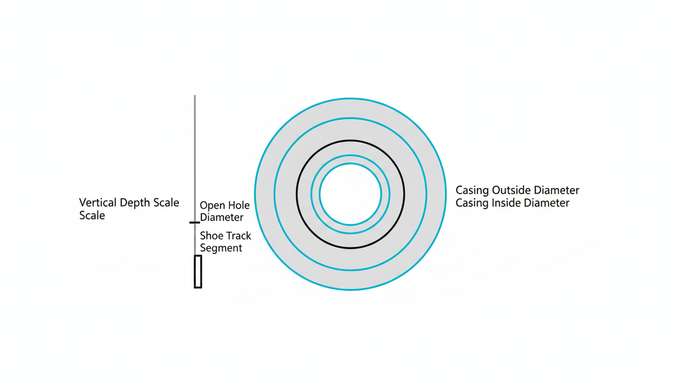
Write every dimension down before touching a formula. Hole size: 12.25 in. Casing: 9.625 in OD, 8.681 in ID. Shoe depth: 8,000 ft. Top of cement: 2,000 ft (the previous casing shoe), so the open hole interval to be cemented is 8,000 − 2,000 = 6,000 ft. Shoe track: 40 ft. Slurry design: Class G cement, 94 lb/sack, specific gravity 3.14, mixed at 5.0 gal of fresh water per sack.
Step 2: Calculate the Annular Capacity and Gross Volume
Cement fills the annulus between the open hole wall and the casing OD. The standard oilfield capacity formula for any annulus, with diameters in inches and capacity in barrels per foot, uses the constant 1029.4 (it comes from converting a cylinder’s cross-sectional area in square inches into barrels per foot):
Capacity (bbl/ft) = (Dhole² − DOD²) / 1029.4
Capacity = (12.25² − 9.625²) / 1029.4 = (150.06 − 92.64) / 1029.4 = 57.42 / 1029.4 = 0.0558 bbl/ft. Over the 6,000 ft open hole interval, the gross (no-excess) annular volume is 6,000 × 0.0558 = 334.7 bbl — the volume you’d need in a perfectly gauge hole with zero washout.

Step 3: Apply the Excess Factor and Add the Shoe Track
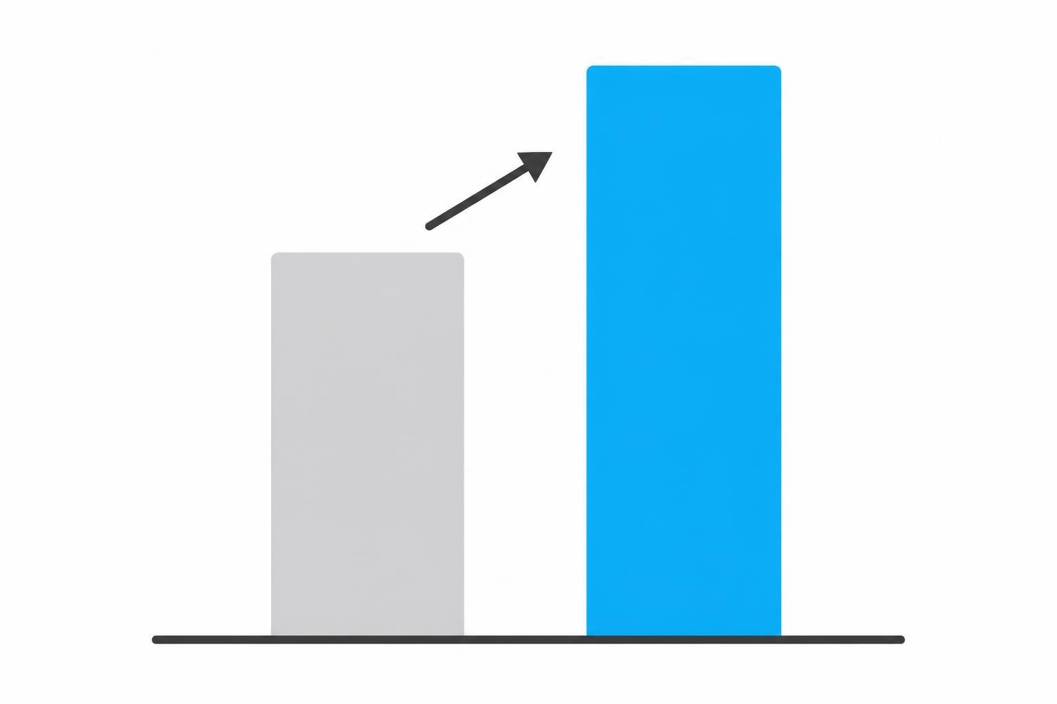
No open hole drills perfectly to gauge. Washouts in shale, breakout in unconsolidated sand, and mud cake thickness all mean the real annulus holds more cement than the bit size alone suggests. A caliper log gives the most accurate excess; without one, 20–50% over gauge is the common planning range for open hole, tightened toward the low end in competent, well-behaved formations and pushed higher in known washout-prone intervals. This example uses a 30% excess:
Excess-adjusted annular volume = 334.7 × 1.30 = 435.1 bbl.
Add the shoe track — the 40 ft of casing below the float collar that stays cement-filled permanently, sized using the casing ID instead of the hole/OD annulus formula, since it’s a simple cylinder: Capacity = ID² / 1029.4 = 8.681² / 1029.4 = 0.0732 bbl/ft. Shoe track volume = 40 × 0.0732 = 2.93 bbl.
Total slurry volume = 435.1 + 2.93 = 438.0 bbl, or 438.0 × 5.615 = 2,460 ft³ once converted to cubic feet for the next step.
Step 4: Convert the Slurry Design to a Yield (Absolute Volume Method)
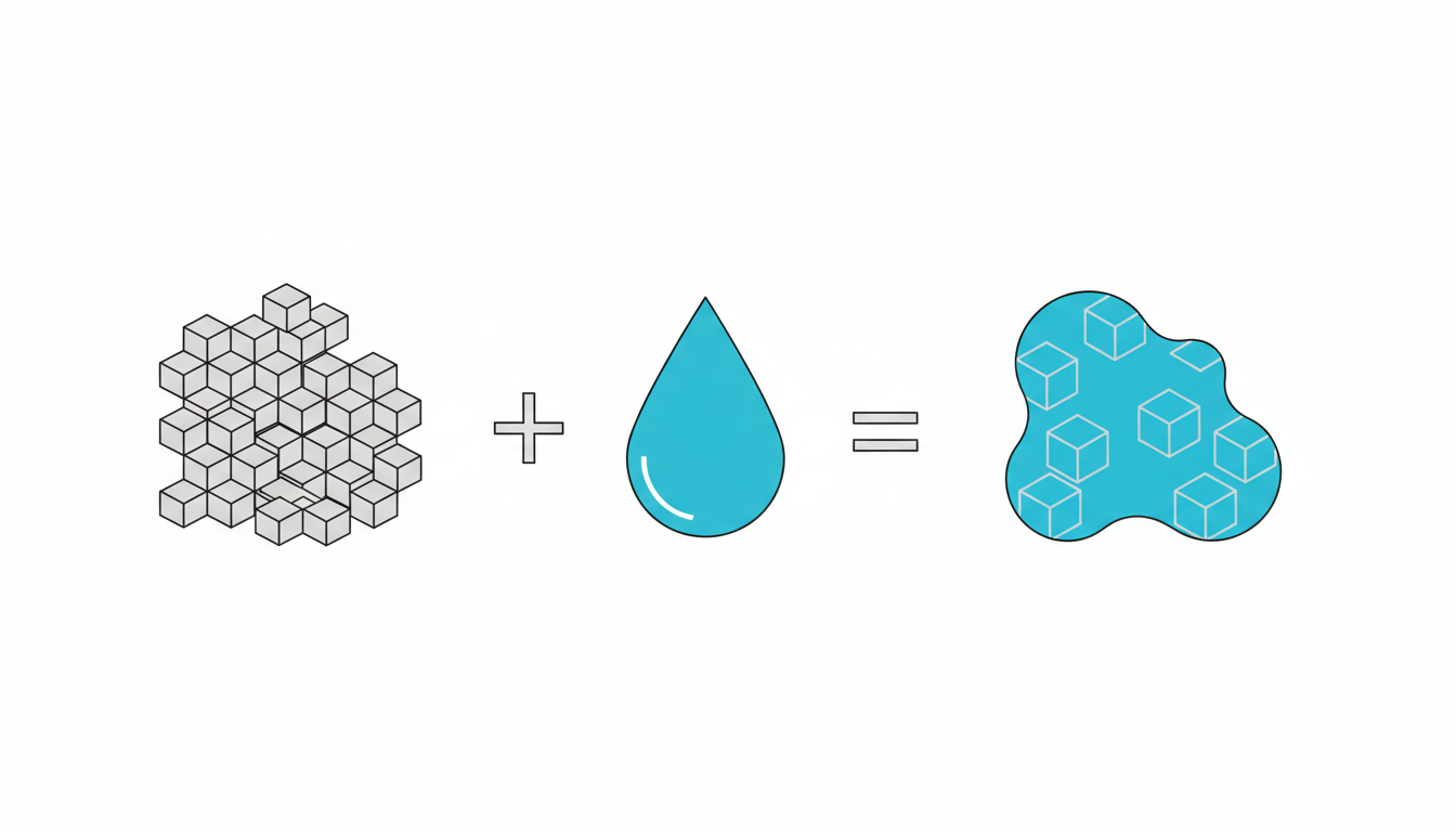
To turn a volume into a sack count, you need the slurry’s yield — how much volume one sack of mixed cement actually produces. Never pull this from a generic table when the lab report is available; derive it directly from the slurry design using the absolute volume method, which simply adds up the physical volume every ingredient occupies:
Absolute volume of cement (ft³/sack) = sack weight (lb) / (SGcement × 62.4 lb/ft³)
Absolute volume of water (ft³/sack) = water (gal/sack) × 0.1337 ft³/gal
For this Class G slurry: cement volume = 94 / (3.14 × 62.4) = 94 / 195.9 = 0.480 ft³/sack. Water volume = 5.0 × 0.1337 = 0.669 ft³/sack. Yield = 0.480 + 0.669 = 1.148 ft³/sack — matching the roughly 1.15 ft³/sack commonly published for neat Class G cement, which is a useful cross-check that the slurry design numbers are sound before you trust them on a live job.
Step 5: Calculate Sacks, Mix Water, and Automate It in Python
Divide total slurry volume by yield to get the sack count: 2,460 / 1.148 = ~2,140 sacks. Multiply sacks by mix water per sack to plan water logistics: 2,140 × 5.0 gal = 10,700 gal, or 10,700 / 42 = ~255 bbl of mix water on location.
Excess factor is the single biggest swing variable in this whole calculation, and it changes every time the open hole interval, mud system or formation changes — which makes this exactly the kind of calculation worth running as a function instead of redoing by hand on every well. Here it is end to end, including a sweep across excess percentages so you can see how sensitive the sack count really is:
import numpy as np

def annular_capacity_bblft(d_hole_in, d_od_in):
    return (d_hole_in**2 - d_od_in**2) / 1029.4

def cylinder_capacity_bblft(d_id_in):
    return d_id_in**2 / 1029.4

def cement_yield_ft3sk(sack_wt_lb, sg_cement, water_galsk, water_density_lbgal=8.33):
    v_cement = sack_wt_lb / (sg_cement * 62.4)
    v_water = water_galsk * 0.1337
    return v_cement + v_water

def cement_job_design(d_hole_in, d_od_in, d_id_in, oh_length_ft, shoe_track_ft,
                       excess_frac, sack_wt_lb, sg_cement, water_galsk):
    cap_ann = annular_capacity_bblft(d_hole_in, d_od_in)
    cap_shoe = cylinder_capacity_bblft(d_id_in)
    vol_ann_bbl = cap_ann * oh_length_ft * (1 + excess_frac)
    vol_shoe_bbl = cap_shoe * shoe_track_ft
    total_bbl = vol_ann_bbl + vol_shoe_bbl
    total_ft3 = total_bbl * 5.615
    yield_ft3sk = cement_yield_ft3sk(sack_wt_lb, sg_cement, water_galsk)
    sacks = total_ft3 / yield_ft3sk
    water_gal = sacks * water_galsk
    return sacks, water_gal / 42.0, total_bbl

# Worked example
sacks, water_bbl, total_bbl = cement_job_design(
    d_hole_in=12.25, d_od_in=9.625, d_id_in=8.681,
    oh_length_ft=6000, shoe_track_ft=40,
    excess_frac=0.30, sack_wt_lb=94, sg_cement=3.14, water_galsk=5.0
)
print(f"Total slurry: {total_bbl:.1f} bbl, Sacks: {sacks:.0f}, Mix water: {water_bbl:.1f} bbl")
# Total slurry: 438.0 bbl, Sacks: 2142, Mix water: 255.0 bbl

# Sensitivity: how hard does excess really swing the sack count?
for excess in (0.10, 0.20, 0.30, 0.40, 0.50):
    sacks, water_bbl, total_bbl = cement_job_design(
        12.25, 9.625, 8.681, 6000, 40, excess, 94, 3.14, 5.0
    )
    print(f"{excess:.0%} excess -> {sacks:.0f} sacks, {total_bbl:.0f} bbl slurry")
Run that sweep once and the lesson is obvious: moving from a conservative 20% excess to a cautious 50% excess on this string adds roughly 500 extra sacks — real money and real logistics, which is exactly why a caliper log that nails down the true excess number pays for itself on anything but the simplest string. Python turns that one-time worked example into a reusable design tool, and a notebook in Jupyter keeps it next to the well plan so you can re-run it the moment the mud report updates the hole size assumption or the lab revises the slurry yield.

Verify the Result
- Cross-check the derived yield against the known reference range for the slurry type — 1.148 ft³/sack for this neat Class G mix lands right where industry references put neat Class G cement (commonly cited around 1.15 ft³/sack at roughly 15.8 ppg), which confirms the absolute-volume math is internally consistent.
- Sanity-check sacks per linear foot of hole: 2,142 sacks over 6,000 ft plus a 40 ft shoe track works out to roughly 0.35 sacks/ft for this 9-5/8 in-in-12.25 in annulus at 30% excess — a figure worth keeping in your head as a reference point for similar strings.
- Confirm the slurry density implied by the mix (total weight per sack ÷ total volume per sack in gallons) lands near the lab report’s stated density; a mismatch of more than a few tenths of a ppg usually means a units slip somewhere in the yield calculation, not a real discrepancy.
Common Pitfalls
- Using casing ID for the annulus and OD for the shoe track. It’s the easiest mixup in the whole calculation — the annulus capacity needs the hole diameter and casing OD; the shoe track needs the casing ID alone, since it’s a plain cylinder.
- Pulling yield from a generic chart instead of the actual slurry design. Additives — extenders, weighting agents, retarders — change both density and yield substantially from the neat-cement numbers in this example; always derive yield from the lab report’s actual water ratio and additive volumes.
- Guessing an excess factor with no caliper or offset-well basis. As the sensitivity sweep shows, excess is the single largest source of error in the whole job design — treat it as a number to justify, not a default to accept.
- Mixing bbl and ft³ partway through. The 5.615 ft³/bbl conversion is easy to apply twice or not at all; keep a single consistent unit system through the sack-count step and the error disappears.
Once the sack count is locked, the next thing worth checking on the same job is whether the planned pump schedule and displacement rate stay inside the fracture gradient at the shoe — see our Eaton’s method fracture gradient tutorial for that calculation — and whether equivalent circulating density during displacement stays inside your mud weight window, covered in the ECD calculation guide. And if your team is still comparing cementing design platforms before committing to one, our roundup of AI cementing design tools for zonal isolation covers what’s actually available right now.
