Gas Gathering Line Sizing: The Weymouth Equation

By Saad Iqbal

A new pad is tied into the gathering system and production is climbing faster than forecast. Someone asks whether the existing 6-inch line can carry it to the compressor station without choking back the wells, and the honest answer requires more than a gut check — it requires knowing, in MMscfd, exactly how much gas that pipe can move between the inlet and outlet pressures you actually have. That calculation has had a name since 1912: the Weymouth equation. It’s still the fastest, most defensible way to size a gas gathering line by hand, and it’s exactly as easy to get wrong as it is to get right if you’re sloppy with the Z-factor.

This tutorial works a real gathering-line sizing problem end to end: pseudo-critical properties, the Dranchuk-Abou-Kassem Z-factor, the Weymouth capacity equation itself, and a Python sweep that turns a single answer into a sizing curve you can hand to the next pad design. It closes with the one sanity check too many sizing memos skip — erosional velocity — because a line that passes the pressure-drop test can still fail from sand cutting or vibration if the gas is moving too fast.

Prerequisites: what you need before you start

• Python 3 with NumPy (or a scientific calculator — the math is all closed-form, just iterative in one spot)
• Inlet and outlet pressures P1, P2 (psia), line length L (miles), and candidate inside diameter D (inches)
• Gas specific gravity γg (air = 1) and average flowing temperature
• A pipeline efficiency factor E — 0.92 is a reasonable default for a clean, fairly new gathering line; use 0.85 or lower for older, liquid-dropout-prone lines
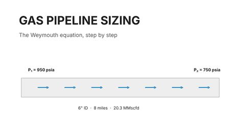
• The worked example below uses: P1 = 950 psia, P2 = 750 psia, L = 8 miles, D = 6.0 in ID, γg = 0.65, T = 70°F, E = 0.92

Step 1: Get the pseudo-critical properties

Everything downstream depends on the gas compressibility factor (Z), and Z depends on the pseudo-reduced temperature and pressure, which depend on the pseudo-critical temperature and pressure. For a sweet, dry gas, Standing’s correlation gets you there from gas gravity alone:

Tpc = 168 + 325γg − 12.5γg² (°R)    Ppc = 677 + 15.0γg − 37.5γg² (psia)

For γg = 0.65: Tpc = 168 + 325(0.65) − 12.5(0.65)² = 374.0 °R, and Ppc = 677 + 15.0(0.65) − 37.5(0.65)² = 670.9 psia. (If the gas has meaningful CO₂ or H₂S, apply the Wichert-Pseudo-Aziz correction before moving on — skipping it is a common source of Z-factor error in sour gathering systems.)

Step 2: Solve for the Z-factor

Use the average line pressure for this calculation — not P1, not P2, but the flow-weighted average: Pavg = (2/3)×(P1 + P2 − P1·P2/(P1+P2)). For our case that’s 853.9 psia. The flowing temperature in Rankine is T = 70 + 459.67 = 529.67 °R. That gives pseudo-reduced values Tpr = T/Tpc = 1.416 and Ppr = Pavg/Ppc = 1.273.

The Dranchuk-Abou-Kassem (1975) correlation solves for Z iteratively from Tpr and Ppr — it’s the same method we used in the gas material balance walkthrough, applied here to pipeline flow instead of a reservoir. The full Python implementation:

import math

def dak_z(Ppr, Tpr):
    A1,A2,A3,A4,A5,A6,A7,A8,A9,A10,A11 = (
        0.3265,-1.0700,-0.5339,0.01569,-0.05165,0.5475,
        -0.7361,0.1844,0.1056,0.6134,0.7210)
    z = 1.0
    for _ in range(200):
        rho_r = 0.27*Ppr/(z*Tpr)
        c1 = A1 + A2/Tpr + A3/Tpr**3 + A4/Tpr**4 + A5/Tpr**5
        c2 = A6 + A7/Tpr + A8/Tpr**2
        c3 = A9*(A7/Tpr + A8/Tpr**2)
        z_new = (1 + c1*rho_r + c2*rho_r**2 - c3*rho_r**5
                 + A10*(1+A11*rho_r**2)*(rho_r**2/Tpr**3)*math.exp(-A11*rho_r**2))
        if abs(z_new - z) < 1e-8:
            z = z_new
            break
        z = z + 0.5*(z_new - z)   # damped update keeps it stable
    return z

Z = dak_z(Ppr=1.273, Tpr=1.416)
print(f"Z = {Z:.4f}")   # Z = 0.8498

For this job, Z = 0.850. Note the damped update step (z + 0.5*(z_new - z)) — a plain fixed-point iteration on this correlation can oscillate near Ppr/Tpr combinations like this one; damping it converges cleanly every time.

Step 3: Apply the Weymouth equation

With Z in hand, the Weymouth capacity equation in US field units is:

Qg = 433.5 × E × (Tb/Pb) × D^2.667 × √[(P1² − P2²) / (γg × T × Z × L)]

where Qg is in scf/day, Tb and Pb are the base (standard) temperature and pressure (520 °R and 14.65 psia here), D is pipe ID in inches, T is flowing temperature in °R, and L is line length in miles. Plugging in P1 = 950, P2 = 750, D = 6.0, γg = 0.65, T = 529.67, Z = 0.850, L = 8, E = 0.92:

P1² − P2² = 902,500 − 562,500 = 340,000. Qg = 433.5 × 0.92 × (520/14.65) × 6.0^2.667 × √[340,000 / (0.65 × 529.67 × 0.850 × 8)] ≈ 20.29 MMscfd.

That's the number that answers the original question: if the new pad's incremental volume pushes total gathering-line throughput past roughly 20 MMscfd at these operating pressures, the 6-inch line is the constraint, not the wells.

Step 4: Automate the diameter sweep

A single answer is useful once. A function is useful every time the next pad gets tied in. Wrapping Step 2 and Step 3 into one callable, and sweeping diameter with Python and Jupyter, turns this into a sizing curve instead of a one-off memo:

def qg_mmscfd(D_in, P1=950.0, P2=750.0, L_miles=8.0,
              gamma_g=0.65, T_F=70.0, E=0.92):
    T_R = T_F + 459.67
    Tpc = 168 + 325*gamma_g - 12.5*gamma_g**2
    Ppc = 677 + 15.0*gamma_g - 37.5*gamma_g**2
    Pavg = (2/3)*(P1 + P2 - (P1*P2)/(P1+P2))
    Z = dak_z(Ppr=Pavg/Ppc, Tpr=T_R/Tpc)
    Tb, Pb = 520.0, 14.65
    Qg = 433.5*E*(Tb/Pb)*(D_in**2.667)*math.sqrt(
        (P1**2-P2**2)/(gamma_g*T_R*Z*L_miles))
    return Qg/1e6

for D in [4.0, 4.5, 6.0, 6.625, 8.0]:
    print(f"{D:5.3f} in ID -> {qg_mmscfd(D):6.2f} MMscfd")

# 4.000 in ID ->   6.88 MMscfd
# 4.500 in ID ->   9.42 MMscfd
# 6.000 in ID ->  20.29 MMscfd
# 6.625 in ID ->  26.43 MMscfd
# 8.000 in ID ->  43.71 MMscfd

That nonlinear jump — going from 6" to 6.625" ID buys 30% more capacity, not the ~10% the diameter increase might suggest — is the direct consequence of the D^2.667 term, and it's the single fact worth remembering from this whole exercise: pipeline capacity is extremely sensitive to diameter, which is exactly why a half-inch difference in nominal pipe size on a new gathering line design is worth arguing about. Feed results like these into pandas for a full gathering-system model, and into Power BI or Looker Studio so the capacity table updates automatically as field pressures change — pairing well with the setup in our virtual flow metering roundup if you're already streaming live wellhead data.

Step 5: Check erosional velocity before you commit to a size

Weymouth tells you what the line can move at a given pressure drop. It says nothing about whether that flow rate will cut or vibrate the pipe. API RP 14E's erosional velocity guideline caps continuous-service gas velocity at v_e = c/√ρ_m, with c = 100 for continuous service in a line without solids-erosion resistant materials, and ρ_m the in-situ gas density in lb/ft³.

At average line conditions (Pavg = 853.9 psia, Z = 0.850, T = 529.67 °R), gas density from the real gas law is ρ_m = Pavg × MW / (Z × R × T) = 3.33 lb/ft³ (MW = 28.97 × γg, R = 10.732 ft³·psia/(lbmol·°R)). That gives v_e = 100/√3.33 ≈ 54.8 ft/s. Converting the 20.29 MMscfd flow to actual volumetric terms at average conditions and dividing by the 6-inch pipe's cross-sectional area gives an actual velocity of about 17.8 ft/s — comfortably under the limit, with headroom for the new pad's volume before erosion becomes a concern.

If your actual velocity comes out above roughly 70-80% of v_e, that's your signal to go up a pipe size even if the Weymouth pressure-drop math still checks out — a gathering line sized purely on pressure drop and run too fast will show up later as sand cutting, noise complaints, or control-valve vibration, not as a Weymouth error.

How to verify it worked

1. Known-Z check: for Tpr and Ppr both near 1.0, Z should sit noticeably below 1.0 (gases depart most from ideal behavior near the critical point); for Tpr well above 2, Z should approach 1.0. Confirm your function behaves that way before trusting it on your real case.
2. Dimensional check: P1² − P2² must use absolute pressures (psia), not gauge — a common error that silently halves or doubles the answer depending on which way it's missed.
3. Order-of-magnitude check: a 6" gathering line at a few hundred psi differential should land in the 10-30 MMscfd range for typical lean gas, not 2 MMscfd or 200 MMscfd — if your result is off by 10x, check that D is in inches (not feet) and L is in miles (not feet).

Common pitfalls

• Using P1 or P2 instead of the flow-weighted average for Ppr. On a line with a large pressure drop, this measurably shifts Z and therefore capacity.
• Ignoring sour gas corrections. Meaningful CO₂ or H₂S content needs a Wichert-Pseudo-Aziz adjustment to Tpc/Ppc before the Z-factor correlation is valid.
• Treating Weymouth as the only check. It's a steady-state, single-phase gas equation — it doesn't catch liquid dropout (use a multiphase correlation for wet gas lines) and it doesn't catch erosional velocity, which is why Step 5 exists.

The Weymouth equation has been the fast, hand-calculable answer to "will this line keep up?" for over a century, and automating it properly — Z-factor, pressure-squared term, erosional check, all in one function — turns a one-time sizing memo into a reusable tool for every pad that gets tied in after this one.