

By Saad Iqbal
At 2:14 a.m., Well 11H burps.
It’s a small thing on the SCADA screen — a cough of gas, a slug of fluid kicked up the tubing, a flowing pressure that spikes for ninety seconds and settles back down. Nobody in the control room looks up. The well is still making gas. The chart still looks fine.
Three weeks later, Well 11H is dead. Not “mechanically failed” dead — drowned. Buried under its own condensate, unable to lift the liquid it is still producing, until the gas simply stops finding a way out. The fix costs a workover rig, a week of lost production, and an uncomfortable conversation about why nobody caught it.
Here’s the uncomfortable part: the well told you. That 2:14 a.m. burp was liquid loading announcing itself, in the one language gas wells speak — pressure and velocity. You just needed to be running the right ten-minute calculation to hear it.
This is a hands-on walkthrough of that calculation: the critical gas velocity Turner equation, the single most useful screening tool for diagnosing liquid loading in a gas well before it kills production. We’ll build it from the ground up, run one fully worked numeric example, and end with a Python script that tracks the trend for you as flowing pressure drifts down over the life of the well.
What Liquid Loading Actually Is, in One Picture
Gas flowing up a wellbore drags liquid droplets — condensate, water, or both — along with it, the same way wind drags raindrops sideways. As long as the gas moves fast enough, the droplets go up. Slow the gas down enough, and gravity wins: droplets start falling back instead of rising, pooling at the bottom of the tubing, adding backpressure, and strangling the well’s own deliverability.
Turner, Hubbard and Dukler worked out the physics in 1969, and it has survived better than almost any other rule-of-thumb in production engineering: there is a minimum gas velocity below which liquid droplets can no longer be carried out of the well. Below it, you’re loading up. Above it, you’re fine. The real question is never “is my well loading up” in some vague sense — it’s “what is my critical velocity, and is my actual velocity above or below it?”
Prerequisites: What You Need Before You Start
Grab these numbers for your own well before working through the steps below. We’ll use one representative example set throughout, so you can check your own arithmetic against ours at every step.
- Tubing inside diameter (d): 2.441 in (2-7/8″, 6.5 lb/ft EUE tubing)
- Flowing wellhead pressure (P): 800 psia
- Flowing temperature (T): 140°F (600°R)
- Gas compressibility factor (Z): 0.88
- Gas specific gravity (γg): 0.75 (air = 1)
- Liquid type: condensate → ρL = 45 lbm/ft³, σ = 20 dynes/cm (use ρL = 67 lbm/ft³, σ = 60 dynes/cm for produced water)
- Actual current gas rate (q_actual): 650 Mscf/d
If you only have surface gas gravity and no lab data on interfacial tension, the Turner condensate/water defaults above are the standard fallback used across the industry — more on why that choice matters in the pitfalls section below.
Step-by-Step: Calculating Critical Gas Velocity with the Turner Equation
Step 1 — Find Your Gas Density at Flowing Conditions

Convert your surface gas gravity into a density at the actual flowing pressure and temperature downhole, using the real gas law:
ρg = 2.70 · γg · P / (Z · T), where P is in psia, T is in °R (°F + 460), and ρg comes out in lbm/ft³.
For our example: ρg = 2.70 × 0.75 × 800 / (0.88 × 600) = 3.068 lbm/ft³.
Why it matters: this is the step most people get wrong, by substituting surface or standard-condition gas density. Gas is far less dense at actual flowing conditions than people expect, and the critical velocity equation is extremely sensitive to this number — it sits under a square root in the denominator.
Step 2 — Apply the Turner-Coleman Critical Velocity Equation
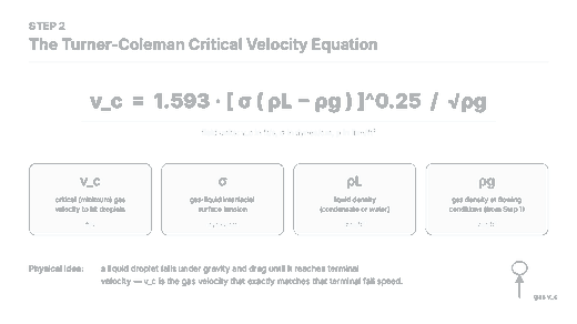
Plug your flowing gas density, liquid density and interfacial tension into the governing equation:
vc = 1.593 × [σ(ρL − ρg)]^0.25 / √ρg
- vc = critical gas velocity, ft/s — the minimum upward velocity needed to keep liquid droplets moving up instead of falling back
- σ = gas-liquid interfacial (surface) tension, dynes/cm
- ρL = liquid density, lbm/ft³
- ρg = gas density at flowing conditions, lbm/ft³ (from Step 1)
For our example: vc = 1.593 × [20 × (45 − 3.068)]^0.25 / √3.068 = 1.593 × (838.6)^0.25 / 1.752 = 1.593 × 5.38 / 1.752 ≈ 4.89 ft/s.
Why it matters: this is the actual physics checkpoint. Everything before it was getting the inputs into field units gas actually obeys; everything after it is just translating this one velocity into something you can compare against a flow rate on your production report.
Step 3 — Convert Critical Velocity to Critical Gas Rate

A velocity alone isn’t directly comparable to the Mscf/d number on your production report — you need the pipe it’s flowing through. Convert using the tubing’s cross-sectional area:
A = (π/4)(d/12)² (ft²), then qc = 3.06 × P × A × vc / (Z × T) (MMscf/d)
For 2.441-in ID tubing: A = (π/4) × (2.441/12)² = 0.0325 ft².
qc = 3.06 × 800 × 0.0325 × 4.89 / (0.88 × 600) = 389.1 / 528 ≈ 0.737 MMscf/d, or 737 Mscf/d.
Why it matters: this is the number you actually compare to real production data. A critical velocity by itself tells you nothing about whether a specific well, at a specific tubing size and pressure, is loading — the critical rate does.
Step 4 — Compare Critical Rate to Actual Rate

Put your actual current gas rate next to the critical rate you just calculated.
- Critical rate, qc: 737 Mscf/d
- Actual rate, q_actual: 650 Mscf/d
- Verdict: q_actual < qc → the well is loading
Why it matters: this is the entire diagnosis, in one comparison. Everything upstream of this step was calculation; this step is judgment. A well producing below its critical rate is actively accumulating liquid, even if the surface data still looks unremarkable — exactly like Well 11H at 2:14 a.m.
Step 5 — Automate It and Track the Trend with Python

A single-point calculation tells you about today. A well lives for years, and its flowing pressure declines the whole time — so the smarter move is to sweep a realistic pressure range and watch exactly where the critical rate crosses your actual rate. The script below does that with numpy; run it in any Python install, or interactively in a Jupyter notebook. If you’d rather not hand-roll your own PVT and flow-correlation helpers, the open-source petropt package on PyPI bundles several, and matplotlib is what drew the trend chart above.
"""
Turner-Coleman critical gas velocity / critical rate calculator.

Computes the critical unloading velocity and critical gas rate for a gas
well across a range of flowing (wellhead) pressures, so you can see the
trend as the well depletes, and flags the pressure at which the well
is predicted to start loading up with liquid.
"""

import numpy as np

# ---- Well & fluid inputs (field units) --------------------------------
d_in     = 2.441     # tubing ID, inches (2-7/8" 6.5 lb/ft EUE tubing)
sg_gas   = 0.75       # gas specific gravity, air = 1
T_f      = 140.0      # flowing (wellhead) temperature, deg F -- held constant across the sweep
Z        = 0.88       # gas compressibility factor at flowing conditions
rho_L    = 45.0       # liquid density, lbm/ft3 (condensate; use ~67 for produced water)
sigma    = 20.0        # gas-liquid interfacial (surface) tension, dynes/cm (condensate; ~60 for water)
q_actual = 0.650       # actual current gas rate, MMscf/d

T_R = T_f + 460.0      # Rankine

# Tubing cross-sectional area, ft^2
A_ft2 = (np.pi / 4.0) * (d_in / 12.0) ** 2

# Sweep of flowing (wellhead) pressures as the well depletes, psia
P = np.linspace(200, 1200, 21)  # psia

# Gas density at flowing conditions, lbm/ft3
rho_g = 2.70 * sg_gas * P / (Z * T_R)

# Turner-Coleman critical velocity, ft/s
v_c = 1.593 * (sigma * (rho_L - rho_g)) ** 0.25 / np.sqrt(rho_g)

# Critical gas rate at that pressure, MMscf/d
q_c = 3.06 * P * A_ft2 * v_c / (Z * T_R)

# Flag: is the well loading up at this pressure (actual < critical)?
is_loading = q_actual < q_c

print(f"{'P (psia)':>10} {'rho_g':>8} {'v_c (ft/s)':>12} {'q_c (MMscf/d)':>15} {'loading?':>9}")
for p, rg, vc, qc, flag in zip(P, rho_g, v_c, q_c, is_loading):
    print(f"{p:10.0f} {rg:8.3f} {vc:12.2f} {qc:15.3f} {str(bool(flag)):>9}")

# Single worked-example point at 800 psia
p0 = 800.0
rho_g0 = 2.70 * sg_gas * p0 / (Z * T_R)
v_c0 = 1.593 * (sigma * (rho_L - rho_g0)) ** 0.25 / np.sqrt(rho_g0)
q_c0 = 3.06 * p0 * A_ft2 * v_c0 / (Z * T_R)
print("\nWorked example at Pwh = 800 psia:")
print(f"  rho_g = {rho_g0:.4f} lbm/ft3")
print(f"  v_c   = {v_c0:.3f} ft/s")
print(f"  q_c   = {q_c0:.3f} MMscf/d  ({q_c0*1000:.0f} Mscf/d)")
print(f"  q_actual = {q_actual*1000:.0f} Mscf/d -> {'LOADING' if q_actual < q_c0 else 'unloaded (OK)'}")

# Find the approximate pressure where q_actual crosses q_c (depletion threshold)
crossing_idx = np.where(np.diff(np.sign(q_actual - q_c)))[0]
if crossing_idx.size:
    i = crossing_idx[0]
    p_lo, p_hi = P[i], P[i + 1]
    q_lo, q_hi = q_c[i] - q_actual, q_c[i + 1] - q_actual
    p_cross = p_lo + (p_hi - p_lo) * (-q_lo) / (q_hi - q_lo)
    print(f"\nApprox. threshold flowing pressure where well starts loading: {p_cross:.0f} psia")
Why it matters: critical rate isn’t fixed — it moves as flowing pressure declines, and this script shows you, numerically, the pressure at which your specific well crosses from fine to loading, so you can see the problem coming weeks before the first burp on SCADA.
Is Your Well Loading Up? Reading the Result
For the inputs above, the result is unambiguous: a critical rate of 737 Mscf/d against an actual rate of 650 Mscf/d means this well is loading right now, and the crossover point in the pressure sweep lands around 617 psia — meaning that as flowing pressure keeps declining below that, the gap only widens unless something changes: smaller tubing, a plunger lift, or another artificial-lift intervention.
Sanity Check
Before you trust any Turner result, run a gut check: critical velocities for typical gas wells on 2-3/8″ to 2-7/8″ tubing almost always land between about 3 and 15 ft/s, and critical rates for those tubing sizes at a few hundred to a couple thousand psia typically land somewhere between a few hundred Mscf/d and a few MMscf/d. If your number is wildly outside that range, re-check your units before you re-check your well.
Common Pitfalls
- Using surface gas gravity instead of flowing-condition gas density. ρg must reflect the actual flowing pressure and temperature at the point you’re evaluating, not standard conditions.
- Mixing up condensate and water fluid properties. Condensate (ρL = 45 lbm/ft³, σ = 20 dynes/cm) and water (ρL = 67 lbm/ft³, σ = 60 dynes/cm) give meaningfully different critical rates; guessing wrong skews the diagnosis in the wrong direction.
- Treating the critical rate as fixed instead of re-checking it as flowing pressure declines. Because qc scales with √P in this model, a well that is comfortably unloaded today can cross into loading purely from declining reservoir pressure — with no change in actual production rate at all. That is exactly what the pressure sweep in Step 5 is for.
Where to Go From Here
The Turner equation is a screening tool, not a verdict — it tells you where to look closer, not what to do about it. If this calculation flags your well, the next question is usually what intervention actually gets you back above critical rate. We’ve covered plunger lift timing in detail in AI Plunger Lift Optimization: Timing the Perfect Cycle, and gone further on combining Turner screening with live SCADA trend detection in AI Liquid Loading Prediction: Beyond Turner’s Model — both worth reading next if this diagnosis matches what you’re seeing in the field.
Run the numbers on your own well today. Ten minutes with a calculator — or the script above — beats finding out at 2:14 a.m.
