

By Saad Iqbal
Seven days before a gas well dies, nothing looks like an emergency. The chart on the SCADA screen shows casing pressure drifting down a little faster than last week. Tubing pressure is doing something similar. A field engineer glancing at the daily report might not even flag it — production is down a few percent, well within the noise band. Then, sometime in the second week, the decline stops being gradual. The well starts heading: pressure builds, slugs of water and condensate lurch up the tubing, rates spike and crash. A few days after that, it goes quiet. No flow, no noise, just a well sitting dead until someone can get a rig or a plunger crew out to it.
That slow slide and sudden death is liquid loading, and it is one of the most common ways a gas well stops paying for itself. It is also, increasingly, a problem being caught earlier by machine learning models reading the same SCADA trends an engineer would glance at — except continuously, at scale, and without waiting for a scheduled check. This is the case for AI liquid loading prediction as something more than a research curiosity, and why the seventy-year-old model most engineers still use to catch it is starting to show its age.
What Liquid Loading Actually Does to a Well
A gas well only stays unloaded if the gas is moving fast enough to carry liquids — condensate, formation water, or both — up and out of the tubing. As reservoir pressure depletes over the life of the well, gas velocity drops. Once it falls below the speed needed to keep droplets airborne, liquid starts falling back instead of lifting out. It accumulates at the bottom of the tubing, adds hydrostatic backpressure against the formation, and chokes the well’s own deliverability. The well produces less gas, which drops velocity further, which loads the well further — a feedback loop that ends, if nothing intervenes, with the well dying completely.
Recovering a loaded-up or dead well is never free. Depending on the well and the field, the fix is some combination of installing a plunger lift, running a velocity string to shrink the effective tubing diameter, or a full workover — and every day the well sits underperforming or fully dead before that intervention happens is production that never gets produced, not just deferred. That combination of intervention cost and lost deliverability is why catching liquid loading early, not just eventually, has real economic weight.
Turner’s Model: A Good Answer to the Wrong-Shaped Question
For decades, the standard tool for this has been the Turner critical velocity model, published in 1969 and still the default check most engineers run by hand or in a spreadsheet. Turner’s model calculates the minimum gas velocity needed to lift the largest stable liquid droplet against gravity, using surface pressure, gas gravity, and liquid density. Compare that critical velocity to the well’s actual velocity at a point in time, and you get a yes-or-no answer: loaded, or not loaded. Li and others later proposed modified droplet-shape assumptions, and models from Turner, Zhang, and Barnea remain the standard critical-velocity correlations engineers reach for first. If you want to see that calculation built out step by step, Gas Well Liquid Loading: Automate the Turner Check walks through automating it in Python.
The trouble is what that calculation leaves out. Turner’s model is a single-point physics check: plug in today’s surface pressure and rate, get today’s answer. It does not look at the trend, does not adapt well to deviated or horizontal trajectories where liquid film behavior departs from the vertical droplet model it was built on, and was calibrated against a specific, fairly narrow dataset of field conditions. That is also why so many modified versions exist — Li-Turner, Zhang, Barnea, Shu-Luo — each trying to patch the same underlying limitation: a static snapshot model standing in for a dynamic, trending phenomenon.
Can Machine Learning Predict Liquid Loading Before Turner’s Model Catches It?
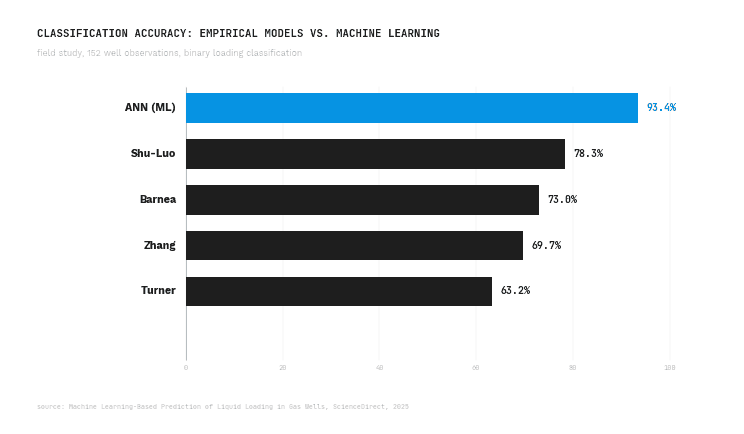
That is the question a growing body of research has been testing directly, and the early answer looks like yes — by a wide margin. A 2025 study published in ScienceDirect, “Machine Learning-Based Prediction of Liquid Loading in Gas Wells for Flow Assurance Management and Production Optimization,” trained feed-forward and cascade-forward artificial neural networks on 152 field observations, using tubing inner diameter, wellhead pressure, gas flow rate, and liquid flow rate as inputs to classify wells as loading or not loading. The neural network reached 93.4% classification accuracy. Turner’s model, run against the same field data, reached 63.2%. The other empirical correlations tested didn’t do dramatically better: Zhang landed at 69.7%, Barnea at 73.0%, and Shu-Luo at 78.3%.
Separately, an SPE paper presented at the 2025 Abu Dhabi International Petroleum Exhibition and Conference, “Artificial Intelligence Enhanced Prediction of Water Loading in Gas Wells: A Data-Driven Alternative to Turner’s Model,” made the same argument from a different angle: that a data-driven model trained on field behavior, rather than a fixed droplet-physics correlation, gives operators a more reliable read on when a well is approaching loaded conditions. The pattern across this research isn’t that Turner’s physics is wrong — the droplet-lift mechanism it describes is real — it’s that a single-point empirical correlation is a blunt instrument for a problem that actually unfolds as a trend over days and weeks.
From a Periodic Check to a Continuous Read on the Well
The practical difference this makes in the field comes down to what data each approach actually uses. A manual Turner check is run when someone runs it — weekly, maybe daily on a watched well, using whatever surface pressure and rate reading was available at that moment. A machine learning model built for gas well deliverability AI instead runs continuously against the SCADA stream, watching how the signals move rather than just where they sit right now:
- Casing and tubing pressure decline rate — not just the pressure itself, but how fast it’s falling and whether that rate is accelerating
- Flowing gradient (dP/dz) — pressure loss along the wellbore, which shifts as liquid holdup increases
- Flow stability signature — the onset of the casing-heading, sawtooth pattern that shows up in rate and pressure data before a well fully unloads-to-loaded
- Gas rate trend against historical decline — deviation from the well’s expected deliverability curve

This is also where the model choice tends to land on random forests, gradient boosting, or neural networks rather than anything exotic — the same family of models used across production-optimization work elsewhere on this site, chosen because they handle the nonlinear, multivariate relationship between pressure trends and loading risk better than a fixed correlation ever could. A related line of published work applied a semi-supervised, temporal-classification approach to minute-level SCADA data from 219 shale gas wells, using a self-attention mechanism to weigh which parts of the pressure trend actually mattered. It classified wells into four severity stages — normal, slight, severe, and flooding — with 98.46% accuracy, and reported flagging loading conditions one to three days earlier than the physical models it was benchmarked against. A one-to-three-day head start is the difference between adjusting choke settings or scheduling a plunger install on your own timeline, and reacting to a well that has already gone intermittent.
What This Looks Like Running: A Trend, Not a Threshold
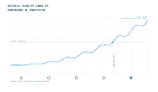
The clearest way to see the difference is side by side. A Turner check is a dot on a timeline — pass or fail, checked every so often. A continuous model is a line that climbs toward a threshold and crosses it while the periodic check is still waiting for its next scheduled run. The gap between when the trend crosses and when the next manual check would have caught it is exactly the early-warning window the research above is measuring.
In practice, teams building this kind of monitoring are pulling SCADA history into pandas, training and validating loading classifiers with scikit-learn, and scoring new SCADA reads against that model on a recurring basis — daily at minimum, ideally against every new polling interval. Field-data platforms like Corva are increasingly where that real-time SCADA stream already lives, which makes them a natural place to wire in a loading-risk score rather than building a separate data pipe from scratch. None of this replaces the physics — a flagged well still gets evaluated the way it always has, including with a Turner-style check as a sanity reference — but it changes when that evaluation happens, from “whenever someone next looks” to “the moment the trend says to.”
What a Gas Well Dying Actually Costs
It’s worth being precise about what’s at stake, because “liquid loading” can sound like a minor operational nuisance until you’ve watched a well go through it. A well that loads up doesn’t just produce a little less gas — it enters the feedback loop described above, where reduced velocity causes more loading, which causes less velocity, until the well is intermittent (flowing in surges, then dying, then unloading and flowing again) or fully dead. Every day in that state is deliverability that is gone, not deferred — gas that a healthy well would have produced and that a dead one simply didn’t. Getting the well back typically means a deliquification intervention: a plunger lift system sized and installed for the well’s specific rate and depth, a velocity string run to shrink tubing diameter and restore critical velocity at lower rates, or, in worse cases, a full workover. Each of those is a planned, budgeted event when it’s caught early — and a more expensive, more urgent one when the well has already died and sat dead waiting for a crew.
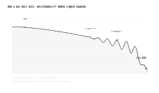
That’s the real case for treating this as a monitoring problem rather than a periodic-checklist problem. The cost driver isn’t the Turner calculation itself — it’s the gap between when loading actually begins and when someone happens to notice.
Where This Fits in a Broader Flow Assurance Stack
Liquid loading prediction doesn’t sit in isolation. It’s one signal among several that a well is drifting out of stable, efficient operation, alongside things like casing heading in gas-lifted wells — if you’re seeing cyclic instability on a gas-lift well rather than a naturally flowing one, AI Gas Lift Instability Detection: Stop Casing Heading covers the related but distinct diagnostic pattern. The point of building liquid loading machine learning into a monitoring stack isn’t to replace engineering judgment — Turner, Li-Turner, and the rest remain useful physical sanity checks, and nobody is deciding to mobilize a plunger crew purely because a classifier crossed a threshold. It’s to make sure that judgment gets applied while there’s still time to choose the response, instead of after the well has already made the choice by going intermittent or dying outright.
The wells worth watching this way are the ones already showing early decline signatures: mature gas wells past peak rate, wells with a history of marginal critical velocity, or wells on fields where deliquification interventions are a recurring, budgeted line item rather than a rare event. For those wells, the question isn’t whether Turner’s model is wrong. It’s whether checking it once a week is still good enough — and for a well whose pressure trend is already telling a different story between checks, the research increasingly says it isn’t.
