Minimum Curvature Method: Automate Directional Drilling Surveys

By Saad Iqbal

The MWD survey lands on the rig floor at 2 a.m.: MD 6,540 ft, inclination 21.6°, azimuth 65.5°. The directional driller needs an answer in the next five minutes — has the dogleg severity over the last 90-ft course crept past the 4°/100ft casing-wear limit, and where did the bit actually go in TVD, North and East? Do the math wrong under time pressure and you either shut down a good slide for nothing or keep sliding through a curve that will tear up the drillstring. This is the exact calculation directional drillers, well planners and MWD engineers run dozens of times a day, and it has one accepted industry answer: the minimum curvature method.

This tutorial walks through the minimum curvature method by hand with a real worked example, then automates it in Python so you never have to redo the arithmetic under a headlamp again.

Prerequisites

• Two consecutive directional survey stations: measured depth (MD), inclination, and azimuth for each
• A scientific calculator or Python 3.10+ (only the standard math module is required)
• Optional for the automation section: pandas for batch-processing a full survey and Matplotlib for plotting the trajectory
• Basic trigonometry — sine, cosine, and inverse cosine

Why the Minimum Curvature Method Wins

Older methods — tangential, balanced tangential, average angle — either overestimate or underestimate wellbore displacement because they treat the path between two stations as straight-line segments. Real wellbores curve continuously between surveys. The minimum curvature method fits a smooth circular arc between the two stations instead, using a ratio factor derived from the dogleg angle to correct the straight-line average. It is the method API and SPE reference texts recommend, and it’s what every commercial well-planning package uses under the hood.

The size of the error is easy to underestimate. Run the tangential method (using only the lower station’s angles) on the same 90-ft course from our worked example, and you get ΔTVD = 83.68 ft, ΔNorth = 13.74 ft, ΔEast = 30.15 ft — versus the minimum curvature values of 84.67 ft, 13.40 ft, and 27.36 ft. The East displacement alone is off by 2.79 ft over one course. That doesn’t sound like much until you chain it across a 300-course lateral: the accumulated position error can put your bit hundreds of feet away from where the survey says it is, which matters enormously for anti-collision, landing in a target zone, or staying inside a spacing unit.

Step 1: Read Two Consecutive Survey Stations

Every course calculation needs six numbers: the measured depth, inclination, and azimuth at the upper station, and the same three values at the lower station. Inclination is measured from vertical (0° = straight down), and azimuth is measured clockwise from true or grid north.

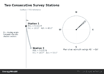
Our worked example uses a build-and-turn course from a real-style curve section:

Station	MD (ft)	Inclination	Azimuth
Upper (1)	6,450.0	18.0°	62.0°
Lower (2)	6,540.0	21.6°	65.5°

Step 2: Calculate the Dogleg Angle and Ratio Factor

The dogleg angle β is the total angular change in wellbore direction between the two stations, found with the spherical law of cosines:

cos(β) = cos(I2 − I1) − sin(I1)·sin(I2)·[1 − cos(A2 − A1)]

The ratio factor RF corrects the straight-line average for the arc’s curvature:

RF = (2 / β) · tan(β / 2)      [β in radians; RF → 1 as β → 0]

Plugging in our two stations: I1 = 18.0°, I2 = 21.6°, A1 = 62.0°, A2 = 65.5°.

• cos(β) = cos(3.6°) − sin(18.0°)·sin(21.6°)·[1 − cos(3.5°)] = 0.99805 − 0.3090 × 0.3681 × 0.001868 ≈ 0.99798
• β = arccos(0.99798) = 3.7887° (0.06612 rad)
• RF = (2 / 0.06612) × tan(0.03306) = 1.0004

The dogleg severity, normalized to degrees per 100 ft of course length (ΔMD = 90 ft here), is:

DLS = β × (100 / ΔMD) = 3.7887° × (100 / 90) = 4.21°/100ft

That’s above a typical 3°/100ft soft-limit but under most 6°/100ft hard casing-wear limits for this hole size — a real “keep sliding, watch it” call, not an automatic shutdown.

Step 3: Calculate ΔTVD, ΔNorth, and ΔEast

With β and RF known, the position increments for the course follow directly:

ΔTVD   = (ΔMD/2)·(cos I1 + cos I2)·RF
ΔNorth = (ΔMD/2)·(sin I1·cos A1 + sin I2·cos A2)·RF
ΔEast  = (ΔMD/2)·(sin I1·sin A1 + sin I2·sin A2)·RF

Working the numbers for our 90-ft course:

Result	Value
ΔMD	90.0 ft
Dogleg angle β	3.7887°
Ratio factor RF	1.0004
ΔTVD	84.67 ft
ΔNorth	13.40 ft
ΔEast	27.36 ft
Dogleg Severity	4.21°/100ft

Quick sanity check: ΔTVD² + horizontal displacement² should be close to ΔMD² for a low-angle course like this (it won’t be exact — that’s exactly what the curvature correction is for). Horizontal displacement here is √(13.40² + 27.36²) = 30.47 ft, and √(84.67² + 30.47²) = 90.0 ft — it closes.

Step 4: Automate It in Python

Here is the full minimum curvature function, verified against the hand calculation above:

import math

def minimum_curvature(md1, inc1, azi1, md2, inc2, azi2):
    """
    Minimum Curvature Method for one course between two survey stations.
    Angles in degrees, depths in feet.
    Returns dMD, dogleg angle, ratio factor, dTVD, dNorth, dEast, DLS/100ft.
    """
    i1, i2 = math.radians(inc1), math.radians(inc2)
    a1, a2 = math.radians(azi1), math.radians(azi2)
    dmd = md2 - md1

    cos_beta = (math.cos(i2 - i1)
                - math.sin(i1) * math.sin(i2) * (1 - math.cos(a2 - a1)))
    cos_beta = max(-1.0, min(1.0, cos_beta))
    beta = math.acos(cos_beta)

    rf = 1.0 if beta < 1e-9 else (2.0 / beta) * math.tan(beta / 2.0)

    dtvd = (dmd / 2.0) * (math.cos(i1) + math.cos(i2)) * rf
    dnorth = (dmd / 2.0) * (math.sin(i1) * math.cos(a1)
                            + math.sin(i2) * math.cos(a2)) * rf
    deast = (dmd / 2.0) * (math.sin(i1) * math.sin(a1)
                           + math.sin(i2) * math.sin(a2)) * rf
    dls = math.degrees(beta) * (100.0 / dmd)

    return {
        "dMD": dmd, "dogleg_deg": math.degrees(beta), "RF": rf,
        "dTVD": dtvd, "dNorth": dnorth, "dEast": deast, "DLS_per_100ft": dls,
    }

result = minimum_curvature(6450.0, 18.0, 62.0, 6540.0, 21.6, 65.5)
for key, value in result.items():
    print(f"{key:>15}: {value:.4f}")

Running this prints dogleg_deg: 3.7887, RF: 1.0004, dTVD: 84.6683, dNorth: 13.4029, dEast: 27.3621, DLS_per_100ft: 4.2096 — matching the hand calculation to four decimal places.

Step 5: Run It Across a Full Survey and Plot the Trajectory

A single course is only useful if it chains into the full wellbore. Loop the function over every consecutive pair of stations, accumulate TVD/North/East, and you get the whole trajectory — this is exactly what a well-planning package does internally, just without the black box:

import pandas as pd

# (MD, Inclination, Azimuth) at each survey station
stations = [
    (6450.0, 18.0, 62.0),
    (6540.0, 21.6, 65.5),
    (6630.0, 25.1, 68.0),
    (6720.0, 28.4, 70.2),
    (6810.0, 31.2, 71.8),
]

md = tvd = north = east = 0.0
rows = [{"MD": stations[0][0], "TVD": 0.0, "North": 0.0, "East": 0.0, "DLS": 0.0}]

for (md1, inc1, azi1), (md2, inc2, azi2) in zip(stations, stations[1:]):
    r = minimum_curvature(md1, inc1, azi1, md2, inc2, azi2)
    tvd += r["dTVD"]
    north += r["dNorth"]
    east += r["dEast"]
    rows.append({"MD": md2, "TVD": round(tvd, 2), "North": round(north, 2),
                 "East": round(east, 2), "DLS": round(r["DLS_per_100ft"], 2)})

df = pd.DataFrame(rows)
print(df)

Feed that DataFrame straight into Matplotlib for a plan-view trajectory plot and a dogleg-severity-versus-depth chart — the two views a directional driller actually looks at during a curve:

Verify Your Result

1. RF should always be ≥ 1.0 and very close to 1.0 for small dogleg angles (under ~5°) — if you get RF < 1.0, check that β is in radians before the tangent step.
2. For a single course, √(ΔTVD² + ΔNorth² + ΔEast²) should equal ΔMD almost exactly (within rounding). If it’s off by more than a few hundredths of a foot, recheck your angle conversions.
3. Cross-check DLS against your rig’s directional driller’s report for the same interval — commercial software (Compass, INSITE, WellPlan) uses this identical formula, so the numbers should match to two decimal places.

Common Pitfalls

• Degrees vs. radians: Python’s math trig functions expect radians. Forgetting to convert inclination and azimuth is the single most common bug in a first implementation.
• β = 0 division: for a perfectly straight course (no change in inclination or azimuth), β is 0 and RF is undefined by the formula — always guard with the if beta < 1e-9 check shown above, or RF collapses to 1.0 anyway in the limit.
• Azimuth wraparound: if a course crosses 000°/360° (e.g., azimuth goes from 358° to 4°), take the shorter angular difference, not the raw subtraction, or the dogleg angle will be wildly overstated.
• Grid vs. true vs. magnetic north: make sure both survey stations and your plan reference the same north — mixing references silently shifts every North/East value.

Tools Used in This Tutorial

• Python — the calculation core, using only the standard library math module
• pandas — for chaining courses into a full survey table
• Matplotlib — for plan-view and dogleg severity charts

Once your trajectory is automated, the next natural step is checking what that wellbore path does to your drilling hydraulics and mud weight window — see our ECD calculation walkthrough for the equivalent circulating density side of the same well, or the kill sheet calculation in Python if you’re building out a full drilling engineering toolkit. Save this minimum curvature function once, and you’ll never hand-calculate a dogleg severity under time pressure again.