
By Saad Iqbal
A pipeline inspector in West Texas once described her job as “reading a patient’s vitals once a year and hoping nothing happened in between.” Ultrasonic thickness surveys, pit gauging, and corrosion coupons tell you the wall thickness on the day someone walks the line with a gauge — and nothing about the eleven months before or after. By the time a scheduled inspection catches a thinning section, corrosion has often already been eating through the pipe for a season. AI well integrity monitoring exists to close that gap, and understanding how it actually works separates a genuinely useful early-warning system from a dashboard full of noise.
Why Periodic Inspection Misses the Failure
Internal corrosion in production tubing and flowlines rarely proceeds at a constant rate. CO2 and H2S partial pressure, water cut, flow velocity, and temperature all swing with production changes, and corrosion rate swings with them — sometimes by an order of magnitude over a few weeks. A single annual ultrasonic reading gives you one point on a curve that actually looks like the chart below: a corrosion rate that AI models can track continuously, catching an acceleration long before the next scheduled survey would.
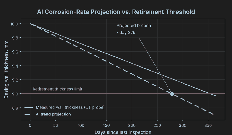
The established way to estimate corrosion rate from first principles is still the de Waard-Milliams model, which relates CO2 corrosion rate to partial pressure, pH, and temperature. It’s a reasonable starting point — but it’s a steady-state equation applied to a well that is never actually at steady state, which is exactly why continuous measurement beats a once-a-year calculation.
What the Sensor Layer Actually Measures
The shift that makes AI well integrity monitoring possible isn’t the AI — it’s the sensors feeding it. Permanently installed ultrasonic wall-thickness sensors (the kind Emerson sells under its Permasense line) report wall loss continuously instead of once a year, and corrosion coupons and ER (electrical resistance) probes add a second, independent read on metal loss rate.

Those readings alone are useful, but noisy — a wireless ultrasonic sensor on a vibrating flowline can drift by fractions of a millimeter from temperature effects and transducer coupling alone. That’s the actual job of the machine learning layer: separating genuine wall loss from sensor noise by cross-referencing the ultrasonic trend against production variables (water cut, flow velocity, CO2/H2S content pulled from produced-fluid analysis) that should move together if the signal is real.
How the Workflow Fits Together
End to end, a working AI well integrity pipeline looks like this:

- Ultrasonic and ER sensors stream wall-thickness and corrosion-rate readings continuously, typically hourly.
- Produced-fluid chemistry and production rate data (water cut, CO2/H2S, velocity) are merged in as context variables.
- A model — often a Bayesian filter or an anomaly-detection algorithm layered on top of a de Waard-Milliams baseline — separates genuine accelerating corrosion from sensor drift and flags statistically significant trend changes.
- Remaining wall thickness is projected forward against the pipe’s minimum allowable wall thickness (per ASME B31.3 or API 570 fitness-for-service rules) to estimate time-to-action, not just current state.
- An integrity engineer reviews flagged assets and schedules an inspection or intervention before the projected remaining-life threshold is reached, instead of waiting for the next calendar-driven survey.
That last point is the real value: the output isn’t “corrosion detected,” it’s a projected date by which action is needed, which is what actually lets an integrity team prioritize a worklist across hundreds of wells instead of treating every flowline as equally urgent.
Can You Build a Lightweight Version Yourself?
If a full continuous-monitoring sensor rollout isn’t in this year’s budget, you can still get meaningful early warning from existing data. Pull coupon and ER probe readings alongside produced-water chemistry into a pandas dataframe, calculate a rolling de Waard-Milliams estimate in Python, and flag any well where the trailing 90-day corrosion rate trend deviates meaningfully from the model’s baseline. Tools like ChatGPT or Claude are genuinely useful here for drafting and checking the statistical trend-detection logic (a simple CUSUM or Z-score change-point test is usually enough) before you hand it to a junior analyst to run weekly. It won’t replace a dedicated sensor network, but it beats waiting for next year’s survey.
What Trips Up a New Deployment?
Three things consistently catch teams off guard:
- Sensor placement bias. A single ultrasonic sensor at the 6 o’clock position on a horizontal flowline will miss top-of-line corrosion entirely in wet-gas service — the model is only as good as where the transducer physically sits.
- Treating every alert as equally urgent. Without the remaining-life projection against a known minimum wall thickness, a 5% rate increase on a thick-walled line and the same increase on a line already near its retirement thickness look identical in a raw alert feed but are wildly different in urgency.
- No chemistry context. A wall-thickness trend without produced-fluid CO2/H2S and water-cut data alongside it can’t distinguish “the well got wetter” from “the sensor drifted,” which is the single most common source of false positives in these systems.
Done well, this turns well integrity from a once-a-year compliance exercise into something closer to continuous monitoring of a patient’s actual vitals. For the sensing side of artificial lift wells covered in a related piece, see AI ESP failure prediction, and for the upstream automation tool landscape more broadly, the integrated asset modelling tools roundup is a good next stop.
