AI Predictive Maintenance for Gas Compressor Failures

By Saad Iqbal

It is 2:14 a.m. when the field supervisor’s phone lights up. A gas lift compressor on high vibration has tripped, the lift gas header pressure is bleeding down, and forty wells on that manifold are backing up oil into the tubing one barrel at a time. By the time a technician reaches the skid, checks the packing, and resets the unit, the field has quietly deferred several hundred barrels of production. Nobody saw it coming because nobody was watching the one signal that had been changing for two weeks: the vibration spectrum on cylinder three.

Reciprocating and screw compressors are the unglamorous backbone of upstream gas handling — they push lift gas into wells, move casing gas to a gathering header, and keep gas plants fed. When one trips unplanned, the damage cascades far past the compressor skid itself. That is exactly the kind of slow-building, high-consequence failure that AI compressor predictive maintenance is built to catch, and it works by teaching a model to read the same vibration data an experienced reliability engineer would read — just continuously, on every unit, instead of on a quarterly walk-around.

Why Compressors Are the Weak Link in Gas Lift and Gathering Systems

A single gas lift compressor commonly serves dozens of wells through a shared header. Compressors also run at higher mechanical stress than most rotating equipment on a pad: reciprocating units have valves opening and closing thousands of times an hour, packing that wears continuously against a moving rod, and cylinders that see full pressure reversal every revolution. Centrifugal and screw units add their own failure modes — oil whirl, surge, bearing wear — but the underlying problem is the same across all three: a mechanical fault shows up in the vibration signature weeks before it shows up as a trip, and most fields still find out only when the trip happens.

The traditional fix — a technician with a handheld vibration meter walking the battery once a month — misses fast-developing faults and can’t tell a real fault from a process transient (a well kicking on and off lift gas looks like a vibration spike too). Continuous, model-scored monitoring closes that gap, but only if the model is built on the right physics, not just a generic anomaly-detection library pointed at a sensor feed.

The Compression Physics a Vibration Model Has to Respect

Before a model can tell you a compressor is behaving abnormally, it needs a normal to compare against — and normal for a reciprocating compressor is governed by polytropic compression. As the piston compresses gas in the cylinder, discharge temperature rises with the compression ratio:

T₂ = T₁ × (P₂/P₁)^((n−1)/n)

• T₁, T₂ — suction and discharge temperature, in absolute units (°R or K)
• P₁, P₂ — suction and discharge pressure, absolute (psia or kPa)
• n — polytropic exponent for the gas (typically 1.20–1.30 for lean, methane-rich associated gas)

Worked example. A single-stage gas lift compressor pulls suction at P₁ = 65 psia and 90°F (550°R), discharging at P₂ = 225 psia, giving a compression ratio r = 3.46. For this gas, n = 1.28:

(n−1)/n = 0.28/1.28 = 0.2188
r^0.2188 = 3.46^0.2188 = 1.312
T₂ = 550 × 1.312 = 721.5°R = 261.8°F

That number matters for two reasons. First, most cylinder discharge-temperature alarms are set somewhere in the 300–350°F range depending on the manufacturer and the gas — so a healthy stage at this ratio should be running with real margin. Second, and more importantly for vibration work: when a discharge valve starts leaking, gas re-expands and recompresses across the same stroke, effective compression work goes up, and both discharge temperature and the vibration signature shift together. A model that only watches vibration and ignores the thermodynamic context will chase noise; one that correlates the two catches real faults faster and with fewer false alarms.

The pressure-volume trace below shows why. A healthy discharge valve produces a sharp, clean corner at the top of the stroke. A worn or leaking valve rounds that corner, lets gas blow back during re-expansion, and traces a visibly different card — a signature a reliability engineer would recognize instantly on a portable analyzer, and one that vibration data captures indirectly as a spike at twice running speed, once per revolution for each cylinder end.

What a Vibration Spectrum Is Actually Telling You

Raw vibration data — an accelerometer time trace — is nearly useless to look at directly. The diagnostic power comes from converting it to the frequency domain with a Fast Fourier Transform (FFT) and reading where the energy shows up relative to the machine’s running speed. For a compressor running at 900 RPM (15 Hz), the diagnostic bands are:

• 1× running speed (15 Hz) — mechanical unbalance, misalignment, or a bent rod
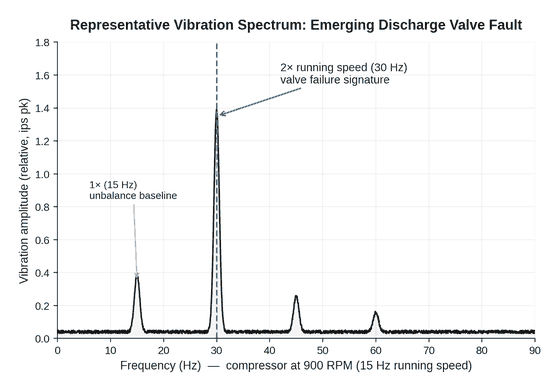
• 2× running speed (30 Hz) — the classic discharge or suction valve fault signature on a reciprocating unit
• 3×, 4× and higher harmonics — looseness, worn crosshead guides, or piston slap
• Sub-synchronous energy (0.4–0.48× running speed) — oil whirl or whip on a centrifugal or screw compressor’s journal bearings

The chart below is representative of exactly the kind of pattern that should trigger a work order, not a shrug: a clean baseline at 1×, and a peak at 2× running speed that has grown steadily over several weeks of trending. On its own, a single elevated reading proves little — process noise, a loose sensor mount, or a nearby pump can all produce a one-off spike. It’s the trend, correlated against load and suction pressure, that separates a developing valve fault from a Tuesday.

How the AI Model Actually Works

Under the marketing language, compressor predictive-maintenance models built by vendors such as those covered in iFactory’s gas compressor monitoring guide follow a fairly consistent recipe, and it’s one you can prototype yourself with a Python stack:

1. Feature extraction. From each accelerometer window, compute RMS amplitude, kurtosis (how “spiky” the signal is — rises sharply with impacting faults like valve slap), crest factor, and the amplitude at each diagnostic harmonic band above.
2. Per-asset baselining. Every compressor is mechanically unique, so the model learns a healthy baseline for that specific unit over its first weeks of run time rather than applying one fleet-wide threshold.
3. Anomaly scoring. An isolation forest or autoencoder scores new readings against the learned baseline, flagging when the feature vector drifts outside the normal envelope — this is what lets the model catch a fault pattern nobody explicitly programmed it to look for.
4. Context correlation. The score is cross-checked against process variables — suction pressure, discharge temperature, load step — so a flag driven by an actual process upset doesn’t get treated the same as one with no operational explanation.

A minimal version of step one — the part every engineer can build and verify by hand before trusting a vendor’s black box — looks like this in Python:

import numpy as np

def vibration_features(signal, fs, rpm, harmonics=(1, 2, 3, 4)):
    """signal: 1D accelerometer trace (g's); fs: sample rate (Hz); rpm: shaft speed."""
    n = len(signal)
    rms = np.sqrt(np.mean(signal**2))
    peak = np.max(np.abs(signal))
    crest_factor = peak / rms
    kurtosis = np.mean((signal - signal.mean())**4) / (np.std(signal)**4)

    freqs = np.fft.rfftfreq(n, d=1/fs)
    spectrum = np.abs(np.fft.rfft(signal)) / n
    running_hz = rpm / 60.0

    harmonic_amps = {}
    for h in harmonics:
        target = h * running_hz
        idx = np.argmin(np.abs(freqs - target))
        harmonic_amps[f"{h}x"] = spectrum[idx]

    return {
        "rms": rms,
        "crest_factor": crest_factor,
        "kurtosis": kurtosis,
        **harmonic_amps,
    }

# Example: 900 RPM compressor, 2 kHz sample rate, 4 seconds of data
# features = vibration_features(accel_trace, fs=2000, rpm=900)
# A 2x-running-speed amplitude that has grown 3-5x over its rolling baseline,
# with kurtosis also trending up, is the pattern worth a work order.

That function is deliberately simple — production systems add windowing, envelope analysis for bearing defect frequencies, and proper harmonic-bin averaging — but the core idea is exactly what it computes: turn a wall of raw samples into the handful of numbers an engineer already knows how to interpret, then let the model watch those numbers continuously instead of once a month.

Reading the Alarm Like an Engineer, Not a Black Box

Even a well-built model needs a severity scale that means something to the person dispatching a technician. The industry reference for that is ISO 10816 / ISO 20816, which buckets broadband vibration velocity into four zones — A (good, as-commissioned), B (acceptable for continuous long-term operation), C (unsatisfactory, tolerable short-term while a repair is planned), and D (vibration high enough that damage is likely). The exact velocity thresholds depend on the machine class and mounting per the ISO 20816 series, but the shape of the decision is always the same:

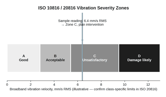
A practical alarm philosophy built on top of that scale: Zone B readings get logged and trended, nothing more. Zone C readings open a work order and trigger a manual review of the spectrum — this is where the AI model’s harmonic breakdown earns its keep, telling the technician what to check before they even open the skid. Zone D readings should already have tripped the unit through hard-wired protection, independent of any model; AI monitoring is there to catch the fault at C, long before it reaches D.

Common Pitfalls

• Sensor placement drift. A vibration signature is only comparable to its own history if the accelerometer stays in the same location and orientation — a sensor knocked loose and remounted six inches away invalidates the baseline.
• Process transients read as faults. A well cycling on and off gas lift, a header pressure swing, or a load-step change all produce vibration spikes that have nothing to do with mechanical condition. This is exactly why context correlation (step 4 above) isn’t optional.
• Cold-start baselines. A newly installed or overhauled compressor needs real run time — typically several weeks across a range of loads — before its “normal” envelope is trustworthy. Trusting an anomaly score in week one is how you get flooded with false positives and a team that starts ignoring the tool.
• Skipping the manual sanity check. Before dispatching a technician on an AI flag alone, pull the actual vibration spectrum or the P-V card if one is available. It takes five minutes and it’s the difference between a confirmed diagnosis and a wasted truck roll.

The Bottom Line

None of this replaces the reliability engineer — it gives them the same diagnostic read they’d get from a handheld analyzer, running continuously on every compressor in the field instead of once a quarter on the units someone remembered to walk. The math behind it is the same polytropic compression and FFT analysis engineers have used for decades; what’s changed is that a model can now watch it around the clock and flag the 2× peak creeping upward two weeks before anyone’s phone rings at 2 a.m.

For the artificial-lift system these compressors feed, the same logic of watching a real physical signal instead of waiting for a trip applies just as directly — see how it plays out for AI dynamometer card diagnostics on rod pumps, for ESP failure prediction from motor current signatures, and for the compressor’s downstream partner in AI gas lift instability detection.