
A well’s monthly report lands in your inbox again and the oil rate has slipped for the sixth month running. Someone in the room asks the question every production engineer eventually has to answer with a number, not a hunch: how much more will this well make, and when does it stop paying for itself? Arps decline curve analysis is the standard way to answer that, and once you have the equation set up correctly it takes seconds to rerun for every well on your lease instead of hours in a spreadsheet.
This tutorial walks through the governing equation, a hand checked example, and a short Python routine you can reuse on any well.
Table of Contents
Prerequisites
- Monthly (or daily) oil rate history for the well, with days on production per period
- A rough idea of the well’s economic limit rate (bbl/d), so you know where the forecast should stop
- Python 3.10+ installed locally, or a hosted notebook such as Jupyter
- Basic comfort with exponents, the hyperbolic equation below is the only math you need

Step 1: Prepare Arps decline curve analysis data
Start with the well’s monthly oil volumes and days on production, not a single “rate” number pulled from a dashboard. A 28 day February and a 31 day January are not comparable unless you divide each month’s oil volume by its own days on figure to get a true bbl/d rate. Skipping this step is the single most common reason a decline fit comes out wrong: a partial month with downtime looks like a sudden decline even when the well behaved normally.

Step 2: Screen Arps decline curve analysis models
Before fitting anything, plot rate versus time on a semi log axis (log rate, linear time). A straight line on that plot means exponential decline (b = 0). A curve that bends means hyperbolic or harmonic decline (0 < b ≤ 1), which is by far the most common shape for unconventional and many conventional oil wells. This chart helps screen candidate models, but curvature alone does not prove a flow regime or unique forecast model, and it’s why skipping straight to a spreadsheet regression on assumed exponential decline is a common way to under- or over forecast reserves.

Step 3: Calculate the Arps decline curve analysis rate
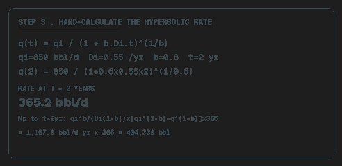
Arps’ (1945) hyperbolic decline equation gives the rate q at any time t:
q(t) = qi / (1 + b·Di·t)^(1/b)where qi is the initial rate (bbl/d), Di is the initial nominal decline rate (1/yr), b is the hyperbolic exponent (0 for exponential, 1 for harmonic, typically 0.3–0.8 for most reservoirs), and t is time in years. Take a well with qi = 850 bbl/d, Di = 0.55 /yr (nominal initial decline), and b = 0.6, and solve for the rate two years out:
q(2) = 850 / (1 + 0.6 × 0.55 × 2)^(1/0.6) = 365.2 bbl/dThe companion cumulative production equation, Np = [qi^b / (Di(1−b))] × [qi^(1−b) − q(t)^(1−b)], is where most hand calculations quietly go wrong: qi is in bbl per day but Di is in 1/year, so the raw result from that formula comes out in bbl/d·yr, not barrels. Multiply by 365 to convert to barrels. For this well, that raw result is 1,107.8 bbl/d·yr, which becomes Np ≈ 404,338 bbl produced over the first two years, not the 1,108 you’d get if you forgot the unit conversion and reported it as is.
Step 4: Automate Arps decline curve analysis in Python
Once the equation and its unit conversion are correct by hand, wrap both functions so you can run every well on your lease in a loop instead of one at a time:
import math

def validate_arps(qi, Di, b, t):
    if not all(math.isfinite(v) for v in (qi, Di, b, t)):
        raise ValueError("Inputs must be finite")
    if qi < 0 or Di < 0 or t < 0 or not 0 <= b <= 1:
        raise ValueError("Require qi, Di, t >= 0 and 0 <= b <= 1")

def arps_rate(qi, Di, b, t):
    """qi in bbl/d, Di in 1/year, t in years."""
    validate_arps(qi, Di, b, t)
    if Di == 0:
        return qi
    if b == 0:
        return qi * math.exp(-Di * t)
    return qi * (1 + b * Di * t) ** (-1 / b)

def arps_cumulative(qi, Di, b, t):
    """Cumulative forecast volume in bbl; use a 365 day year."""
    validate_arps(qi, Di, b, t)
    if Di == 0:
        integral = qi * t
    elif b == 0:
        integral = qi * (-math.expm1(-Di * t)) / Di
    elif b == 1:
        integral = qi * math.log1p(Di * t) / Di
    else:
        exponent = (b - 1) / b
        integral = qi * (-math.expm1(exponent * math.log1p(b * Di * t))) / (Di * (1 - b))
    return integral * 365

qi, Di, b = 850.0, 0.55, 0.6
for t in range(6):
    q = arps_rate(qi, Di, b, t)
    Np = arps_cumulative(qi, Di, b, t)
    print(f"t={t} yr  q={q:.1f} bbl/d  Np={Np:,.0f} bbl")

# At t=2: q=365.2 bbl/d, Np=404,338 bbl
# b=0 uses exponential decline; b=1 uses harmonic decline.
The self contained Python routine handles exponential, hyperbolic and harmonic Arps decline curve analysis, including zero nominal decline. It checks basic input domains and uses separate cumulative expressions to avoid division by zero at b = 0 or b = 1. For the stated hyperbolic example, the independently checked result is q(2) = 365.2348 bbl/d and cumulative volume 404,337.52 bbl.

Step 5: Apply Arps decline curve analysis forecast limits
Extend the same loop until the rate crosses your well’s economic limit, the rate at which revenue no longer covers lifting cost, commonly in the 10–30 bbl/d range for a stripper well, but always specific to your operating cost structure. That crossing point, not an arbitrary end date, is what defines the well’s remaining economic life and its estimated ultimate recovery (EUR).

Arps decline curve analysis verification and pitfalls
For the well used in this Arps decline curve analysis, reproduce q(2) = 365.2 bbl/d and Np(2) = 404,338 bbl after rounding. Di and t must use the same time unit, with the appropriate conversion from rate to volume. Check the reservoir flow regime and operating changes before extending a fitted curve. If a terminal exponential decline is used, select a documented terminal decline rate and switch when the instantaneous nominal hyperbolic decline reaches it.
For deeper reservoir characterization to pair with a decline forecast, see our guide to building a Horner plot for pressure buildup analysis in Python, and for turning a forecast into an operating point, our nodal analysis in Python tutorial. If your well also needs a PVT check before you trust the rate data, our companion tutorial on calculating bubble point pressure with Standing’s correlation covers that next step.
Arps decline curve analysis interpretation and forecast checks
Nominal decline is not effective percentage decline. Di is an instantaneous rate of change normalized by rate. For an exponential model, annual effective decline equals 1 − exp(−Di). Thus Di = 0.55/year corresponds to about 42.3% effective decline over one year in the exponential case. For the hyperbolic example, the first year rate ratio also depends on b. Do not label every nominal Di as the same annual percentage fall in production.
Choose the time and rate basis explicitly. An on production day rate describes capacity while the well is flowing. A calendar day rate includes downtime. Either can be useful if used consistently, but they answer different questions. If Arps decline curve analysis fits flowing day rates, apply a documented uptime assumption when forecasting calendar volume. Do not adjust for downtime twice by fitting an already normalized calendar rate and multiplying it by another availability factor.
Fit a representative operating period. Stimulation, artificial lift changes, choke restrictions and allocation changes can alter the production trend. Record these events before selecting the fitting window. A smooth curve through all history can mix different operating systems. Arps decline curve analysis assumes a suitable decline regime and sufficiently consistent conditions; a good numerical fit does not make an inappropriate interval physically valid.
Validate on later observations. Fit an earlier portion of the selected history and compare the forecast with later measurements. Inspect rate and cumulative errors, rather than only the regression residual on training data. Try reasonable alternative fitting windows. If the forecast changes dramatically after a small window adjustment, report that uncertainty instead of selecting the most optimistic result.
Define cumulative volume from the correct origin. The routine integrates from the model time origin to t. When forecasting remaining production from a later date, subtract cumulative volume at the forecast start from cumulative volume at its end. Add actual historical production separately when calculating a total recovery estimate. Otherwise Arps decline curve analysis can double count already produced barrels.
Control the long term tail. The instantaneous nominal hyperbolic decline is Di/(1 + b·Di·t). A terminal exponential segment can be introduced when this reaches a defensible terminal rate. Match rate continuously at the switch and integrate both segments consistently. A harmonic curve has an unbounded infinite time integral, so the economic and operating limits remain essential even when its short term fit looks good.
Distinguish forecast volume from booked reserves. Arps decline curve analysis produces a conditional production forecast. Recoverable and economic quantities depend on operating constraints, costs, prices and the applicable evaluation framework. The example does not classify reserves. State the forecast horizon and economic limit, and compare multiple plausible cases before using the result for a development decision.
Keep the uncertainty visible. Present the selected qi, Di and b with the fitting interval, units and forecast start date. Compare alternative models and uptime assumptions. A model with more adjustable parameters can match history better without predicting the future better. Retain the raw data and calculation version so another engineer can reproduce the same Arps decline curve analysis and understand why the selected forecast was preferred.
