

By Saad Iqbal
The well has been flowing steadily for thirty days at 850 STB/d when production shuts it in for a 48-hour pressure buildup test. Forty-eight hours later, a memory gauge hands the engineer thirteen pressure-versus-time pairs and one question that costs real money either way: is this well damaged enough to justify a matrix acid job, or is the low rate just a reservoir quality problem no stimulation will fix? The answer lives inside a single straight line on a semi-log plot — the Horner plot — and the two numbers it gives you, permeability and skin factor, are exactly what a completions engineer needs before signing off on a job ticket.
This tutorial builds a complete Horner plot analysis by hand with a verified worked example, then automates the whole workflow in Python.
Prerequisites
- A pressure buildup dataset: shut-in time Δt and corresponding shut-in bottomhole pressure Pws for each reading
- Flow rate q, formation volume factor B, viscosity μ, and net pay thickness h from before shut-in
- Porosity φ, total compressibility ct, and wellbore radius rw for the skin calculation
- Python 3.10+ with NumPy for the straight-line regression and Matplotlib for plotting
Why the Horner Plot Still Runs the Show
A pressure buildup test works because shutting in a well is mathematically equivalent to superimposing an injection well at the same rate on top of the producer — the pressure response during the buildup follows a predictable semi-log relationship with the “Horner time ratio” (tp + Δt) / Δt, where tp is the flowing time before shut-in. Plot shut-in pressure Pws against the log of that ratio, and the middle-time region (once wellbore storage effects die out and before boundary effects show up) falls on a straight line. The slope of that line is directly proportional to permeability, and the pressure drop right at the start of shut-in versus where that line extrapolates tells you the skin — how much extra pressure drop is happening right at the wellbore that reservoir quality alone doesn’t explain.
Step 1: Record the Buildup Test Data
Our worked example: a well produced q = 850 STB/d for tp = 720 hours (30 days) before shut-in, with B = 1.20 rb/STB, μ = 1.5 cp, and h = 42 ft of net pay. Reservoir properties from core and log data: φ = 0.18, ct = 1.2×10⁻⁵ psi⁻¹, rw = 0.328 ft.

The memory gauge recorded shut-in pressure Pws at thirteen shut-in times Δt:
| Δt (hr) | (tp+Δt)/Δt | Pws (psi) |
| 0.5 | 1441.0 | 4,357.64 |
| 1.0 | 721.0 | 4,404.52 |
| 1.5 | 481.0 | 4,431.92 |
| 2.0 | 361.0 | 4,451.35 |
| 3.0 | 241.0 | 4,478.70 |
| 4.0 | 181.0 | 4,498.08 |
| 6.0 | 121.0 | 4,525.34 |
| 8.0 | 91.0 | 4,544.63 |
| 12.0 | 61.0 | 4,571.71 |
| 18.0 | 41.0 | 4,598.61 |
| 24.0 | 31.0 | 4,617.53 |
| 36.0 | 21.0 | 4,643.90 |
| 48.0 | 16.0 | 4,662.31 |
Step 2: Plot Pws Against log[(tp+Δt)/Δt] and Fit the Straight Line
The governing equation for the Horner plot is:
Pws = P* − m·log10[(tp + Δt) / Δt]where P* is the false (extrapolated) pressure at infinite shut-in time and m is the slope, in psi per log cycle. The first two or three points (Δt = 0.5 and sometimes 1.0 hr) are usually still inside the wellbore storage-dominated region and get excluded from the straight-line fit — using them would bias the slope. Fitting a least-squares line to the ten points from Δt = 2 hr onward:
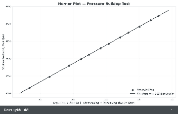
- Slope m = 155.88 psi/cycle
- Extrapolated pressure P* = 4,850.0 psi
Step 3: Calculate Permeability
Permeability comes directly from the slope:
m = 162.6 · q · B · μ / (k · h)
k = 162.6 · q · B · μ / (m · h)
k = 162.6 × 850 × 1.20 × 1.5 / (155.88 × 42)
k = 38.0 md
That’s a decent mid-permeability sandstone — not tight, but nothing that would explain a well underperforming its type curve on reservoir quality alone.
Step 4: Calculate Skin Factor and Flow Efficiency
Read P1hr directly off the fitted straight line at Δt = 1 hr (4,404.52 psi here), and take Pwf as the last flowing bottomhole pressure recorded right before shut-in (3,071.70 psi in this test):
s = 1.151 × [ (P1hr − Pwf)/m − log10(k / (φ·μ·ct·rw²)) + 3.23 ]
s = 1.151 × [ (4404.52 − 3071.70)/155.88 − log10(38.0 / (0.18×1.5×1.2e-5×0.328²)) + 3.23 ]
s = 4.31
A skin of +4.31 is real, positive damage — consistent with drilling mud invasion or perforation restriction, and exactly the kind of number that justifies a stimulation job. Flow efficiency converts that into a single “how much better could this well do” figure:
FE = (P* − Pwf − 0.87·m·s) / (P* − Pwf) = 0.67
A flow efficiency of 0.67 means this well is only delivering about two-thirds of the rate an undamaged completion would give at the same drawdown — a strong economic case for acidizing before drilling an infill location that doesn’t need one.
Step 5: Automate the Full Analysis in Python
Here’s the complete, verified workflow — from raw buildup data to k, skin, P*, and flow efficiency — using NumPy‘s least-squares fit instead of eyeballing a straight line on graph paper:
import numpy as np
import math

# Well and fluid properties
q, B, mu, h = 850.0, 1.20, 1.5, 42.0        # STB/d, rb/STB, cp, ft
phi, ct, rw = 0.18, 1.2e-5, 0.328           # fraction, 1/psi, ft
tp = 720.0                                   # hours flowing before shut-in
Pwf = 3071.70                                # psi, flowing BHP at shut-in

# Buildup data: shut-in time (hr), shut-in pressure (psi)
dt = np.array([0.5, 1, 1.5, 2, 3, 4, 6, 8, 12, 18, 24, 36, 48])
Pws = np.array([4357.64, 4404.52, 4431.92, 4451.35, 4478.70, 4498.08,
                4525.34, 4544.63, 4571.71, 4598.61, 4617.53, 4643.90, 4662.31])

horner_ratio = (tp + dt) / dt
x = np.log10(horner_ratio)

# Fit only the middle-time straight-line region (skip early wellbore storage)
mask = dt >= 2
slope, intercept = np.polyfit(x[mask], Pws[mask], 1)
m, Pstar = -slope, intercept

k = 162.6 * q * B * mu / (m * h)
P1hr = Pstar - m * math.log10((tp + 1) / 1)
skin = 1.151 * ((P1hr - Pwf) / m
                - math.log10(k / (phi * mu * ct * rw**2)) + 3.23)
FE = (Pstar - Pwf - 0.87 * m * skin) / (Pstar - Pwf)

print(f"m     = {m:.2f} psi/cycle")
print(f"k     = {k:.2f} md")
print(f"P*    = {Pstar:.2f} psi")
print(f"skin  = {skin:.2f}")
print(f"FE    = {FE:.3f}")
This prints m = 155.88 psi/cycle, k = 38.00 md, P* = 4850.00 psi, skin = 4.31, FE = 0.671 — matching the hand calculation exactly, and ready to plot with Matplotlib in three more lines using plt.semilogx(horner_ratio, Pws, "o").
Verify Your Result
- P* should always be greater than the highest Pws you measured — if it isn’t, your straight-line fit is using the wrong points or the data has a sign error.
- A positive skin (s > 0) means damage; a negative skin (commonly −2 to −5) indicates a stimulated or naturally fractured well. Flow efficiency should sit between roughly 0 and 1 for a damaged well and can exceed 1 for a stimulated one — a negative FE means something upstream is wrong.
- Re-run the fit using only Δt ≥ 3 hr and only Δt ≥ 4 hr — if k and skin shift by more than a few percent between the two, your straight-line region hasn’t fully stabilized and you need more late-time data.
Common Pitfalls
- Including wellbore-storage-affected points: the earliest shut-in readings are almost never on the true semi-log straight line. Fitting them in drags your slope — and therefore your permeability — off.
- Wrong sign convention on the slope: Pws decreases as the Horner ratio decreases, so the raw regression slope is negative; m itself is defined as positive. Forgetting the sign flip silently produces a negative permeability.
- Using average reservoir pressure instead of Pwf: the skin equation needs the actual flowing bottomhole pressure at the instant of shut-in, not a static or average pressure — mixing them up produces a skin factor that’s off by a large, confusing margin.
- Ignoring boundary effects at late time: if the last few points curve away from the straight line (up or down), the well may be seeing a reservoir boundary or an offset well’s pressure interference — exclude those points from the permeability fit too.
Tools Used in This Tutorial
- Python — the calculation environment
- NumPy —
polyfitfor the semi-log least-squares regression - Matplotlib — for the semi-log Horner plot itself
Once you know the skin and permeability, the natural next question is what rate this well should actually be making — run those numbers through our nodal analysis in Python tutorial to solve for the operating point against your VLP curve, or check how AI predicts ESP failures if the well is on artificial lift and the damage you just quantified is compounding a lift problem. A verified skin and permeability from a five-minute Python script beats a guess every time a stimulation budget is on the line.
