
By Saad Iqbal
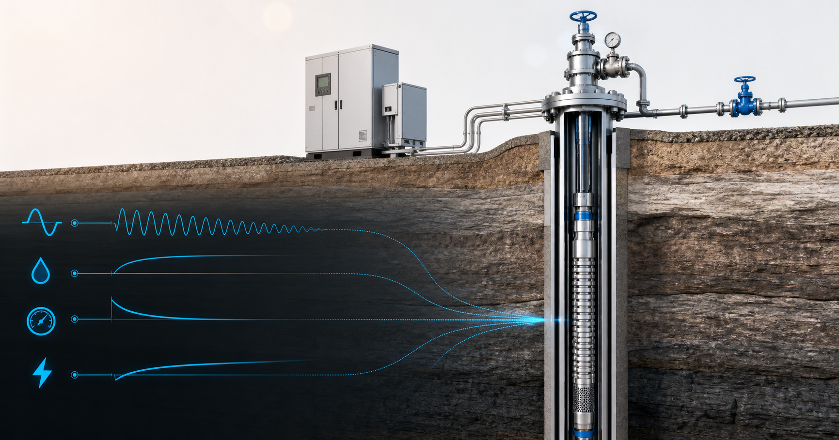
An ESP is running at 50 Hz, the well is stable, and operations wants to know what will happen at 55 Hz before anyone changes the variable-speed drive. The quick answer is not “ten percent more of everything.” Flow changes roughly with speed, head with speed squared, and power with speed cubed. That last relationship is why a small frequency increase can consume motor margin much faster than expected.
This tutorial builds an ESP affinity laws calculator in Python. We will calculate a transparent screening case, sweep frequencies from 45 to 60 Hz, and identify what still needs to be checked against the vendor pump curve and the well’s inflow/outflow model.
Prerequisites
- Python 3.10+ with
pandasandmatplotlib - Baseline frequency: 50 Hz
- Baseline flow: 2,000 BPD
- Baseline head: 24 ft per stage
- Number of stages: 120
- Baseline input power: 80 hp
- Produced-fluid specific gravity: 0.85
- Target frequency: 55 Hz
- The manufacturer’s pump curve, recommended operating range, motor rating and cable limits for the actual installation
The Hydraulic Institute’s pump-curve guidance states the speed affinity relationships and their constant-efficiency assumption. SLB’s ESP overview is a useful reference for the downhole and surface components being modelled. Treat the calculator below as a screening tool, not a substitute for the manufacturer’s stage curve or a calibrated well model.
Step 1: Validate the ESP baseline inputs
Start from one operating point that you trust. Use stabilized rate, frequency and electrical data collected at the same time. Do not mix yesterday’s rate with today’s frequency or a design-stage head copied from a different pump.
Our base case is 2,000 BPD at 50 Hz. The pump has 120 stages producing 24 ft per stage at the selected baseline point, so total baseline head is:
H1 = 24 ft/stage × 120 stages = 2,880 ft
With fluid specific gravity SG = 0.85, the corresponding ideal differential pressure is:
ΔP1 = H1 × SG / 2.31 = 2,880 × 0.85 / 2.31 = 1,059.7 psi
Head is energy per unit weight, so the affinity calculation should be done in head first. Convert head to pressure afterward using the actual mixture density. If free gas changes materially with intake pressure, a fixed specific gravity becomes a weak assumption and a multiphase ESP model is required.

Step 2: Apply the three ESP affinity laws
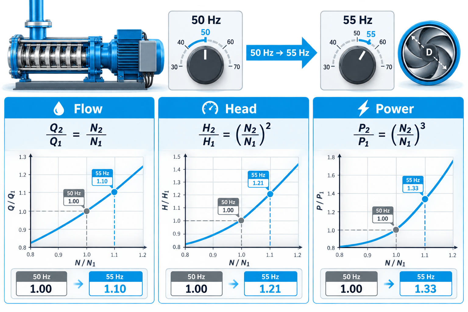
For the same pump and impeller geometry, with efficiency assumed unchanged, the speed relationships are:
Q2/Q1 = N2/N1
H2/H1 = (N2/N1)²
P2/P1 = (N2/N1)³
Here Q is flow rate, H is head, P is input power and N is rotational speed. For an induction motor controlled by a variable-speed drive, frequency is commonly used as the practical speed ratio for a first-pass calculation:
r = N2/N1 ≈ f2/f1 = 55/50 = 1.10
The equations move an entire pump curve; they do not independently determine the well’s final stabilized rate. The actual operating point is where the shifted pump curve interacts with the system and reservoir. That is why an affinity-law result should later be checked with a calibrated IPR-VLP nodal analysis.
What the speed ratio does—and does not—represent
For a first-pass VSD calculation, the frequency ratio is used as the speed ratio because synchronous motor speed changes with electrical frequency. The real motor speed also depends on pole count and slip. That distinction normally does not invalidate a modest screening calculation, but it matters when the analysis is expected to reproduce measured shaft speed precisely.
The similarity assumption also expects geometrically similar flow through the same pump and roughly similar efficiency. An ESP operating near its best-efficiency region may follow the shifted curve reasonably for a limited frequency change. A pump already affected by free gas, high viscosity, scale, worn stages or recirculation can depart materially from the ideal relationship. The calculator therefore predicts how the reference point scales; it does not diagnose the condition of the equipment.
Step 3: Work the 55 Hz example by hand
With r = 1.10, predicted flow becomes:
Q2 = 2,000 × 1.10 = 2,200 BPD
Head per stage becomes 24 × 1.10² = 29.04 ft/stage. Across 120 stages:
H2 = 2,880 × 1.10² = 3,484.8 ft
Using the same fluid specific gravity:
ΔP2 = 3,484.8 × 0.85 / 2.31 = 1,282.3 psi
Power rises much faster:
P2 = 80 × 1.10³ = 106.48 hp
The frequency increased by 10%, but the screening power requirement increased by 33.1%. Before increasing speed, compare that result with the motor nameplate, VSD current limit, cable rating and expected temperature. Also confirm that the shifted operating point remains inside the manufacturer’s recommended operating range rather than simply chasing more rate.

Step 4: Automate the ESP frequency sweep in Python
The following script calculates every integer frequency from 45 to 60 Hz. It deliberately keeps the math visible and exports a CSV that can be reviewed independently.
import pandas as pd
import matplotlib.pyplot as plt

f1 = 50.0              # Hz
q1 = 2000.0            # BPD
head_stage_1 = 24.0    # ft/stage
stages = 120
power1 = 80.0          # hp
sg = 0.85

rows = []
for f2 in range(45, 61):
    ratio = f2 / f1
    q2 = q1 * ratio
    head_stage_2 = head_stage_1 * ratio**2
    head_total_2 = head_stage_2 * stages
    pressure_2 = head_total_2 * sg / 2.31
    power_2 = power1 * ratio**3
    rows.append({
        "frequency_hz": f2,
        "speed_ratio": ratio,
        "flow_bpd": q2,
        "head_ft": head_total_2,
        "pressure_psi": pressure_2,
        "power_hp": power_2,
    })

df = pd.DataFrame(rows)
print(df.loc[df["frequency_hz"].isin([45, 50, 55, 60])].round(2))
df.to_csv("esp_affinity_sensitivity.csv", index=False)

fig, axes = plt.subplots(2, 2, figsize=(10, 7), sharex=True)
for ax, column, label in [
    (axes[0, 0], "flow_bpd", "Flow (BPD)"),
    (axes[0, 1], "head_ft", "Total head (ft)"),
    (axes[1, 0], "pressure_psi", "Differential pressure (psi)"),
    (axes[1, 1], "power_hp", "Input power (hp)"),
]:
    ax.plot(df["frequency_hz"], df[column], marker="o")
    ax.axvline(50, color="gray", linestyle="--", label="Baseline")
    ax.axvline(55, color="#0693e3", linestyle="--", label="Scenario")
    ax.set_ylabel(label)
    ax.grid(alpha=0.25)

axes[1, 0].set_xlabel("Frequency (Hz)")
axes[1, 1].set_xlabel("Frequency (Hz)")
plt.tight_layout()
plt.show()
A basic sanity check is the 55 Hz row: 2,200 BPD, 3,484.8 ft total head, about 1,282 psi and 106.48 hp. If your script does not reproduce those values, check the frequency ratio and exponents before using it.
Turn the sensitivity table into an operating decision
Add columns for the actual motor limit, maximum allowable current, minimum and maximum recommended pump rate, and the drawdown predicted by the nodal model. A simple Boolean flag can then identify scenarios that deserve further review. Do not let the script issue a VSD setpoint automatically; its job is to make assumptions and constraints visible to the engineer and operator.
After an approved change, compare stabilized measured rate, intake pressure, motor current and temperature with the prediction. If the rate response is smaller than expected while current rises sharply, return to the pump curve, gas fraction and well inflow instead of forcing the frequency higher. That comparison converts a one-time calculator into a feedback loop and creates better baseline data for the next optimization cycle.

Expected result and engineering sanity checks
The calculator should make the nonlinear trade-off obvious: raising frequency modestly increases the theoretical rate, but it increases head faster and power fastest. The 55 Hz result is a screening point, not a control instruction.
- Pump curve: shift the full manufacturer curve and find the new intersection with the system curve.
- Operating envelope: keep the point inside the recommended operating range and check thrust limits.
- Motor and cable: compare predicted load with nameplate power, current, voltage drop and thermal limits.
- Gas and viscosity: affinity laws assume similar hydraulic behavior; gas interference and viscosity can materially change performance and efficiency.
- Reservoir response: confirm the well can deliver the predicted liquid without unacceptable drawdown, gas production or sand risk.
Common pitfalls
- Treating the affinity result as the final production rate. The well and surface system determine the operating point.
- Assuming efficiency is constant over a large speed change. Use the vendor curve and a calibrated model for the decision.
- Ignoring the cubic power relationship. A frequency change that looks small can consume motor margin quickly.
Conclusion
An ESP affinity laws calculator is valuable because it turns a proposed frequency change into an auditable first-pass estimate. Use it to screen scenarios, identify motor-load risk and decide which cases deserve a full pump-curve and nodal-analysis review. For condition monitoring after the change, continue with the EnergyMindAI guide to ESP failure prediction using operating data.
Archive the input snapshot, CSV and approved operating change together. That small record makes the result reproducible and lets the next engineer distinguish a modelling assumption from a value measured in the field.
