Bit Nozzle TFA Calculator in Python

By Saad Iqbal

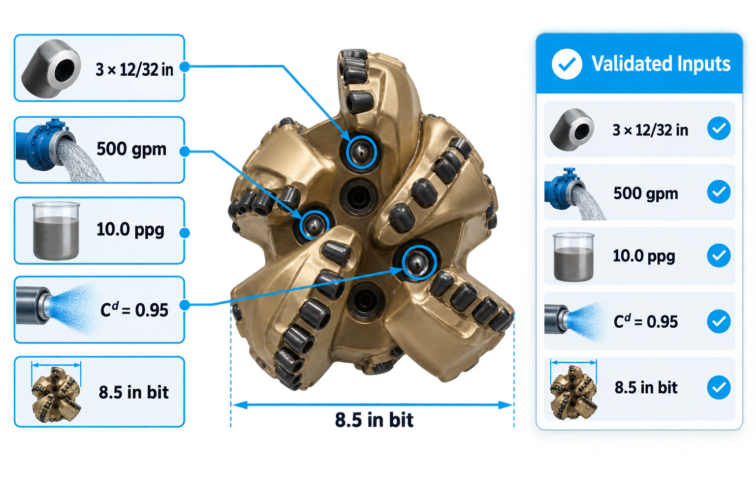
A drilling program shows three 12/32-inch bit nozzles, 500 gpm and 10.0 ppg mud. The pump can deliver the flow, but the team still needs to know how much pressure will be consumed across the bit and whether the selected nozzles create a credible hydraulic load. That calculation is simple enough to do by hand and repetitive enough to automate.

This tutorial builds a bit nozzle TFA calculator in Python. We will calculate total flow area, jet velocity, nozzle pressure loss, bit hydraulic horsepower and hydraulic horsepower per square inch, then run a nozzle-size sensitivity without hiding the governing equations.

SLB’s drilling-hydraulics data dictionary identifies bit nozzle TFA and jet velocity as core calculated channels. Baker Hughes lists optimized nozzle selection and bit hydraulic horsepower among the capabilities of its drilling engineering software. The Navi-Drill motor handbook also emphasizes checking flow, differential pressure and bypass/nozzle selections against the specific motor limits.

Step 1: Validate nozzle and circulating inputs

Confirm whether nozzle sizes are recorded in thirty-seconds of an inch. A “12” nozzle normally means 12/32 in, not 12 mm and not 0.12 in. Verify the number of installed nozzles and whether all are the same size.

Use the circulating flow and mud weight expected at the calculation point. The discharge coefficient accounts for real contraction and losses through the nozzle; it should come from the selected nozzle model or an approved engineering assumption. We use Cd = 0.95 only to make the worked example reproducible.

Finally, collect the full system pressure budget. Bit nozzle pressure loss is only one part of standpipe pressure. A nozzle selection that looks attractive in isolation can exceed the rig or motor limit once surface, pipe, motor and annular losses are added.

Step 2: Calculate total flow area

Convert the nozzle designation to diameter in inches:

d = 12/32 = 0.375 in

The circular flow area of one nozzle is:

A = πd²/4

For d = 0.375 in:

A = π × 0.375² / 4 = 0.11045 in²

Total flow area is the sum of the individual nozzle areas:

TFA = 3 × 0.11045 = 0.33134 in²

For mixed nozzle sizes, calculate each area separately and sum them. Do not average the diameters first; area varies with diameter squared.

Why TFA is the controlling geometry

At fixed pump flow, total area determines the average velocity through the nozzle set. Pressure loss then changes approximately with the inverse square of TFA. This makes nozzle selection sensitive: a small diameter change can produce a much larger pressure change than intuition based on diameter alone suggests.

TFA does not describe nozzle orientation, stand-off, cutter cleaning or flow distribution across the bit face. Two bits with the same TFA can perform differently because their nozzle placement and blade geometry are different. Use the calculator for the hydraulic arithmetic, then keep the selection within the bit supplier’s approved nozzle configuration.

Step 3: Calculate velocity, pressure loss, HHP and HSI

With flow Q in gpm and TFA in square inches, average nozzle jet velocity is:

V = 0.32086 Q / TFA

For 500 gpm and 0.33134 in²:

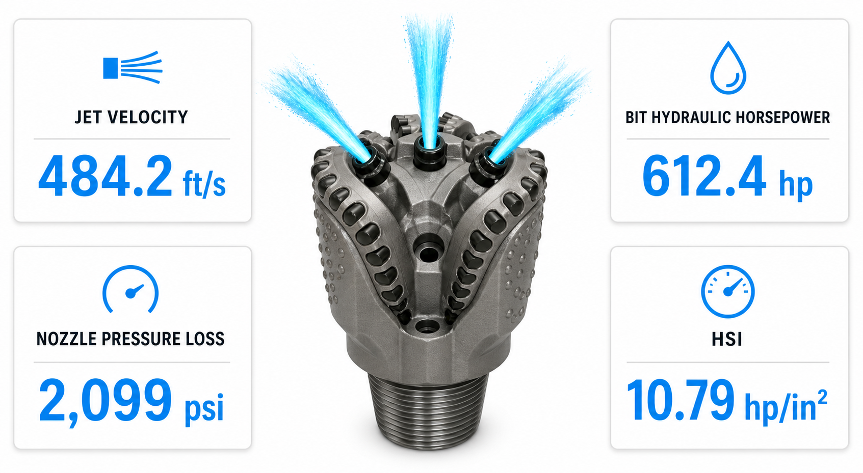
V = 0.32086 × 500 / 0.33134 = 484.2 ft/s

A field-unit form of the incompressible orifice equation gives nozzle pressure loss:

ΔP = 8.32 × 10⁻⁵ MW Q² / (Cd² TFA²)

where ΔP is psi, MW is mud weight in ppg, Q is gpm, Cd is dimensionless and TFA is in². Substitution gives:

ΔP = 8.32 × 10⁻⁵ × 10.0 × 500² / (0.95² × 0.33134²) = 2,099 psi

Bit hydraulic horsepower is:

HHP = ΔP Q / 1714 = 2,099 × 500 / 1714 = 612.4 hp

For an 8.5-in bit, face area is πD²/4 = 56.75 in². Hydraulic horsepower per square inch is:

HSI = HHP / (πD²/4) = 612.4 / 56.75 = 10.79 hp/in²

These are idealized nozzle results. They do not prove that the rig can supply the total pressure or that the bit, motor and formation will tolerate the hydraulic loading. Add every other system loss and compare the total with the pump curve and approved operating limits.

Step 4: Automate the nozzle sensitivity in Python

The script below evaluates equal three-nozzle combinations from 10/32 to 16/32 in. It applies the same equations used by hand and prints a transparent comparison table.

import math
import pandas as pd
import matplotlib.pyplot as plt

flow_gpm = 500.0
mud_weight_ppg = 10.0
cd = 0.95
bit_diameter_in = 8.5
nozzle_count = 3

rows = []
for size_32 in range(10, 17):
    diameter_in = size_32 / 32.0
    one_area_in2 = math.pi * diameter_in**2 / 4.0
    tfa_in2 = nozzle_count * one_area_in2
    velocity_fts = 0.32086 * flow_gpm / tfa_in2
    nozzle_dp_psi = (
        8.32e-5 * mud_weight_ppg * flow_gpm**2
        / (cd**2 * tfa_in2**2)
    )
    hhp = nozzle_dp_psi * flow_gpm / 1714.0
    bit_area_in2 = math.pi * bit_diameter_in**2 / 4.0
    hsi = hhp / bit_area_in2
    rows.append({
        "nozzles": f"{nozzle_count} x {size_32}/32 in",
        "tfa_in2": tfa_in2,
        "jet_velocity_fts": velocity_fts,
        "nozzle_dp_psi": nozzle_dp_psi,
        "hhp": hhp,
        "hsi_hp_per_in2": hsi,
    })

df = pd.DataFrame(rows)
print(df.round(2).to_string(index=False))
df.to_csv("bit_nozzle_sensitivity.csv", index=False)

fig, axes = plt.subplots(1, 2, figsize=(11, 4))
axes[0].plot(df["tfa_in2"], df["jet_velocity_fts"], marker="o")
axes[0].set_xlabel("TFA (in²)")
axes[0].set_ylabel("Jet velocity (ft/s)")
axes[0].grid(alpha=0.25)

axes[1].plot(df["tfa_in2"], df["nozzle_dp_psi"], marker="o")
axes[1].set_xlabel("TFA (in²)")
axes[1].set_ylabel("Nozzle pressure loss (psi)")
axes[1].grid(alpha=0.25)

plt.tight_layout()
plt.show()

The 12/32 row is the sanity check: TFA ≈ 0.33134 in², V ≈ 484.2 ft/s, ΔP ≈ 2,099 psi, HHP ≈ 612.4 hp and HSI ≈ 10.79 hp/in². If those values do not reproduce, inspect nozzle count, the 32nds conversion and the squared TFA term.

Build the complete circulating-pressure budget

Extend the exported table with pressure losses from surface equipment, drillpipe, drill collars or BHA, downhole motor and annulus. Sum those values with the nozzle pressure loss to estimate standpipe pressure at each candidate flow rate. Keep a separate margin below the approved maximum rather than treating the equipment limit as a normal operating target.

If a motor contains a rotor bypass nozzle or a circulation sub, the flow split must be handled explicitly. The total rig flow is not necessarily the flow passing through the bit. Use the motor technical data sheet and manufacturer method to calculate the power-section flow and bit flow before applying the nozzle equations.

Finally, repeat the calculation at the low and high ends of the planned mud-weight and flow ranges. A single nominal case can hide the condition that controls the job. The sensitivity table is most valuable when it shows which combination first consumes pump-pressure margin or moves the motor outside its approved flow and differential-pressure envelope.

Expected result and engineering sanity checks

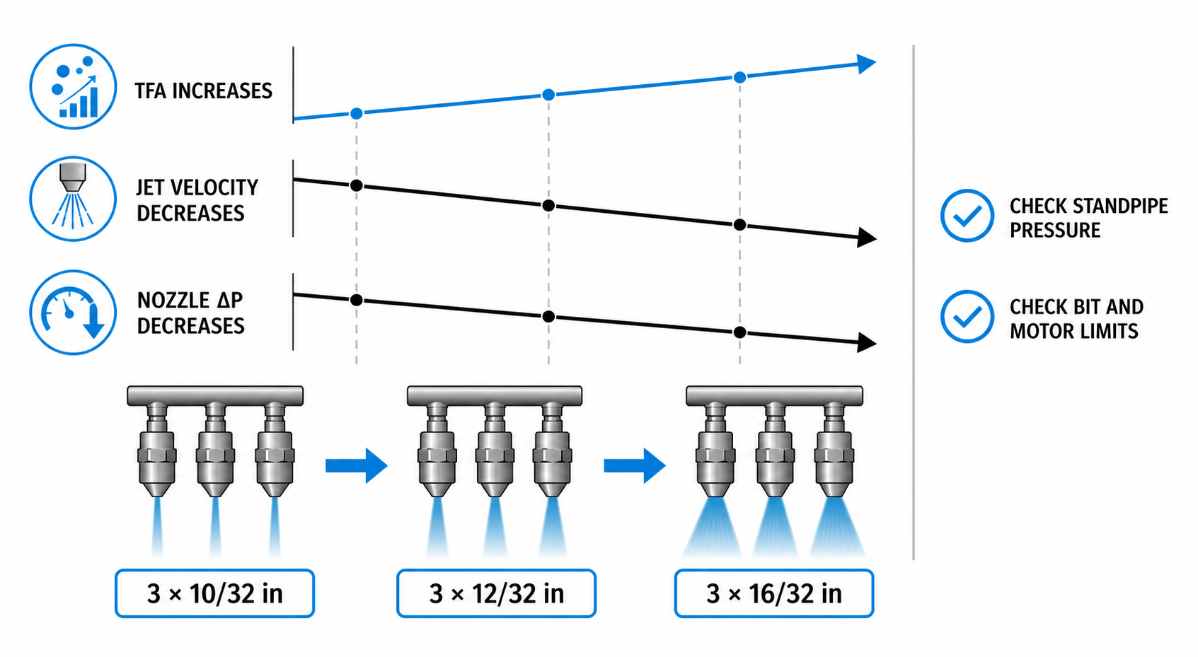
The sensitivity should show that larger nozzles increase TFA and reduce both velocity and nozzle pressure loss at fixed flow. Smaller nozzles do the opposite. The preferred selection is not automatically the smallest nozzle: the full drilling system needs adequate hole cleaning, available standpipe pressure, acceptable motor differential pressure and bit hydraulics within approved limits.

• Pressure budget: add surface, drillstring, motor, bit and annular losses before comparing with maximum standpipe pressure.
• Motor compatibility: confirm flow and differential pressure with the motor technical data sheet.
• Bit specification: use the bit supplier’s permitted nozzle combinations and operating recommendations.
• ECD and losses: changing flow to recover hydraulics also changes annular pressure loss and ECD. Recheck the safe window with the EnergyMindAI ECD calculator.

Common pitfalls

1. Treating a 12 nozzle as 0.12 in. Oilfield nozzle designations are commonly expressed in 32nds of an inch.
2. Averaging mixed diameters. Calculate each circular area and sum the areas.
3. Comparing nozzle ΔP directly with the standpipe limit. The pump must also overcome every other circulating-system loss.

Conclusion

A bit nozzle TFA calculator makes nozzle selection faster and auditable, but the result must remain inside the real pump, motor and bit envelopes. Use the sensitivity to narrow the options, then confirm them in the approved drilling-hydraulics model. For the mechanical side of the plan, compare the outcome with EnergyMindAI’s guide to torque and drag optimization tools, and monitor for loss risk using the lost-circulation prediction workflow.

Save the nozzle configuration, assumptions and sensitivity table with the drilling program. A short auditable record prevents unit mistakes and gives the morning tour a clear basis for any later hydraulics change.

---