AI Lost Circulation Prediction While Drilling

By Saad Iqbal

It’s 2:47 a.m. on an exploration well, and the mud logger’s screen is throwing numbers that don’t quite add up. Standpipe pressure is holding steady. Rate of penetration looks normal. But the pit volume totalizer has quietly bled off eleven barrels in the last twenty minutes, and nobody on the rig floor has flagged it yet. By the time the pit-volume alarm finally trips — the same fixed threshold this rig has run for fifteen years — the well has lost 140 barrels of synthetic-based mud into a fractured stringer nobody had mapped. The kill-and-cure job that follows costs two days and a mid-six-figure mud bill.

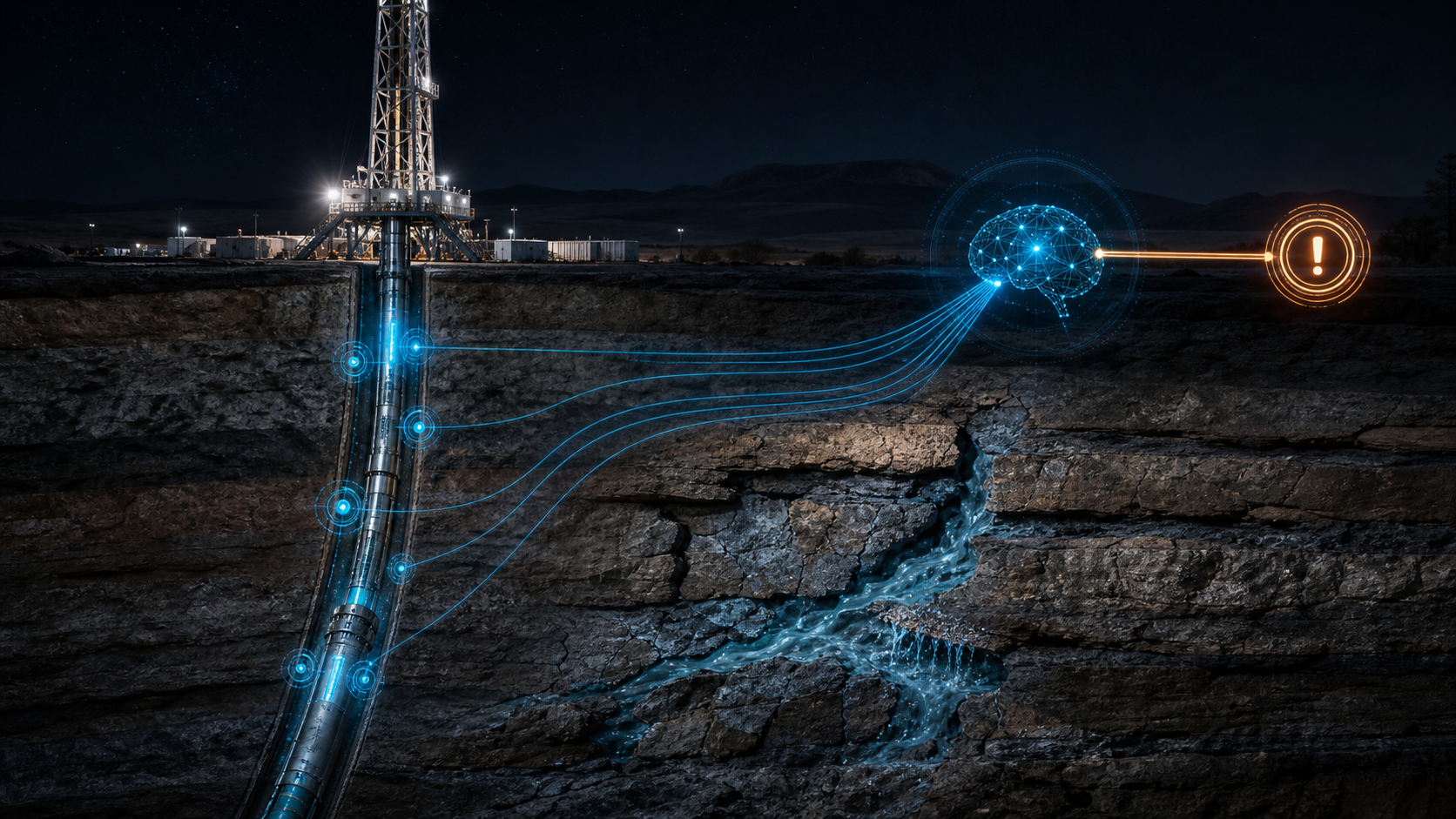
That two-day gap between “the losses started” and “the alarm noticed” is exactly what lost circulation prediction models are built to close. Not by drilling differently. By reading the same surface data every rig floor already has, faster and more suspiciously than a threshold alarm ever will.

What Lost Circulation Actually Costs

Lost circulation isn’t a rare, exotic failure — it’s one of the most persistent line items in the drilling non-productive-time ledger, especially in fractured or vugular carbonate formations. A 2022 review in PMC on lost circulation control technology in fractured formations puts a number on it: Chinese national oil companies alone report direct economic losses exceeding 10 billion yuan per year from lost circulation, and CNPC’s own operations log more than 4,000 lost days annually from the problem — over two-thirds of all recorded “drilling complex incident” time on their wells (PMC, 2022). Scale that pattern across every operator drilling through fractured carbonates, salt, or depleted sands, and the honest answer to “what does lost circulation cost the industry” is: more than almost anything else that isn’t a blowout.

The frustrating part is that the physics isn’t mysterious. Losses happen when the equivalent circulating density in the wellbore exceeds what the formation can take:

ECD (ppg) = MW (ppg) + [APL / (0.052 x TVD (ft))]

where MW is your static mud weight, APL is the annular pressure loss from circulating friction, TVD is true vertical depth, and 0.052 converts psi/ft into ppg. When ECD creeps past the local fracture gradient — commonly estimated with Eaton’s equation, FG = Pp/D + (σv/D − Pp/D) x [ν/(1−ν)], using pore pressure Pp, overburden stress σv, depth D, and Poisson’s ratio ν — you open fractures and mud starts disappearing. Every mud engineer on the planet knows this equation. The problem was never understanding the physics. It was seeing the trend in time to do anything about it, buried as it is in six or seven noisy channels updating every few seconds.

How Machine Learning Actually Predicts It

This is where lost circulation prediction models earn their keep, and it’s worth being precise about what they actually do, because “AI predicts drilling problems” is vague enough to be useless. The published models don’t replace the ECD/fracture-gradient physics above — they watch for the multivariate pattern that precedes a breach of it, across the same surface channels a mud logger already has on screen.

A study published in ACS Omega and indexed on PMC trained several algorithms — K-nearest neighbors, support vector machines, and random forest — on flow rate, standpipe pressure, weight on bit, ROP, RPM, and surface torque, using active pit volume as the signal to reconstruct. On a held-out well, K-NN alone hit an R of 0.90 with an RMSE of 0.17; across a seven-well test split it reached R = 0.94, outperforming both SVM (R = 0.53) and random forest (R = 0.84) (PMC / ACS Omega). Separately, a particle-swarm-optimized backpropagation neural network (PSO-BP) trained on pit volume, standpipe pressure, flow-in/flow-out delta, hook load, ROP, mud density, and wellbore inclination reported 95.6% classification accuracy in Nature Scientific Reports — and in one field validation example, correctly bracketed an actual loss zone at 2,723 m depth by predicting a loss window of 2,686–2,756 m (Nature Scientific Reports).

Notice what’s missing from both input lists: nothing exotic. No new downhole sub, no extra sensor package. Flow rate, SPP, pit volume, WOB, ROP, RPM, torque, hook load, mud weight, inclination — every one of those already streams off the rig’s existing surface instrumentation. The model’s edge isn’t better data. It’s noticing a six-variable deviation that a human watching one trend line at a time, at 3 a.m., on hour eleven of a tour, is never going to catch as fast.

Reading the Early-Warning Signal

Here’s what that looks like in practice. A slow, real loss doesn’t announce itself with a pit-volume cliff — it announces itself as a subtle divergence between what standpipe pressure is doing and what pit volume is doing, minutes before the trend is large enough to trip a fixed threshold.

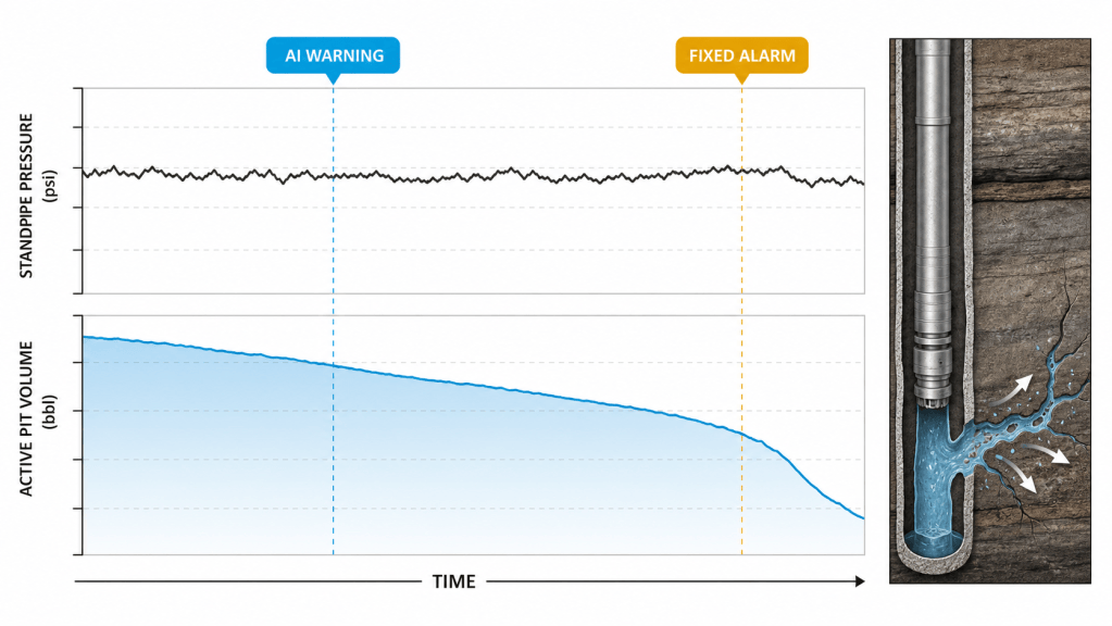
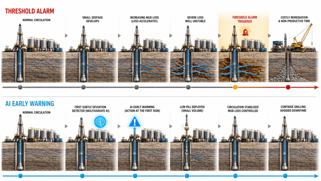
That gap between “the pattern started” and “the threshold tripped” is the entire value proposition. A fixed pit-volume alarm is, by design, reactive — it can only fire after enough fluid is already gone to cross a line someone drew on a chart years ago. A model trained on the joint behavior of six or seven channels can flag the same event while the loss is still small enough to manage with an LCM pill instead of a full lost-circulation kill job.

What Changes on the Rig Floor

None of this replaces the mud engineer’s judgment — it changes what they’re judging. Instead of watching seven raw trend lines and mentally correlating them, the workflow becomes a four-stage loop: the real-time data stream feeds the model continuously, the model scores loss probability and estimated time-to-event, the engineer reviews any flagged deviation against what they know about the formation, and only then does a mitigation action — reducing ECD, pulling back ROP, staging LCM — actually get called.

That last point matters more than the accuracy numbers. A model that’s 95% accurate but only fires after losses are already unmanageable is worse than useless — it’s a false sense of security. The studies worth paying attention to are the ones measured on lead time, not just classification accuracy: minutes or hours of runway before the event, not just a correct label after the fact.

Where This Is Already Running

You don’t need a research grant to get this on a live well. Real-time drilling analytics platforms already ingest the exact channel list these studies use and layer anomaly detection or predictive scoring on top of it. Corva streams and contextualizes live rig data for exactly this kind of early-warning application; Petrolink‘s real-time operations software does similar surface-data aggregation and analytics across rig fleets; and Kelvin builds autonomous control applications that can act on these signals rather than just display them. None of these are a substitute for a competent mud engineer. They’re a substitute for staring at seven charts at once and hoping your pattern recognition holds up at hour eleven of the tour.

If you’re chasing well control risk instead of fluid losses, the same early-warning logic — reading a multivariate deviation minutes before a fixed alarm fires — is exactly what we walked through in AI Kick Detection: How Machine Learning Beats the Clock, where models catch a well control event up to 100 minutes ahead of a conventional pit-gain alarm. And if the surface data you’re watching is vibration rather than volume, How AI Predicts Stick-Slip Before It Wrecks Your BHA covers the same six-channel-surface-data philosophy applied to protecting your bottom-hole assembly instead of your mud system.

The Bottom Line

Lost circulation prediction isn’t a new physics discovery — the ECD and fracture gradient equations haven’t changed. What’s changed is that a model can now watch the six or seven variables that determine whether you’re about to breach that fracture gradient, continuously, without getting tired at 3 a.m. That’s the entire pitch: not a smarter well, a faster read on the well you already have. Given that CNPC alone is losing 4,000 days a year to this problem, a few extra minutes of lead time on every well adds up to a lot of mud that stays in the hole instead of the formation.