
By Saad Iqbal
Every coiled tubing job, someone on the crew is supposed to update the string’s fatigue log — pull the reel’s bend history, flip through the vendor’s cumulative-damage spreadsheet, add this job’s cycles, check whether the string crossed the retirement line. In practice it gets done in a rush between jobs, on a laptop with three other spreadsheets open, and the number that decides whether a string goes back down hole is only as good as whoever last updated it. This tutorial builds a coiled tubing fatigue life calculation you can trust: the governing equation, one full worked example by hand so you know what “right” looks like, and then a Python tracker that does the arithmetic for you on every job going forward.
The stakes for getting this wrong run in both directions. Retire a string too early on a hunch and you’re leaving thousands of feet of usable pipe on the shelf. Run it too long on an out-of-date spreadsheet and you’re one bad bend away from a parted string downhole — a fishing job at best, a well control incident at worst. Neither failure mode comes from bad engineering; both come from the update never happening because the calculation was too tedious to do consistently. That’s the problem this tutorial actually solves.
Prerequisites
- Python 3.10+ installed, with pandas available (
pip install pandas) — see Python and pandas. - Your CT string’s fatigue curve constants (fatigue strength coefficient and exponent) from your service company’s engineering data, or a published model such as BSEE’s public-domain CTLIFE2 methodology. This tutorial uses illustrative constants — swap in your own before you trust the output for a real string.
- A per-job log: bend cycles applied and the estimated bending/pressure stress amplitude for each job, from your job engineering plan.
- The string’s cumulative damage entering today — carried forward from its last BOL (beginning-of-life) reset or its last known inspection point.
Step 1 — Read the string’s S-N fatigue curve
Coiled tubing fatigue is low-cycle bending fatigue: every trip over the reel and the injector’s gooseneck flexes the pipe wall past its elastic limit, a little more each time depending on bend radius and internal pressure. The relationship between how hard you bend it (stress amplitude) and how many cycles it takes to crack (cycles to failure) follows the classic power-law shape known as Basquin’s relation:
sigma_a = sigma_f * (2 * N_f) ** b
- sigma_a — bending stress amplitude for this bend location, in your fatigue curve’s index units (from your CT engineering software, driven by bend radius, wall thickness and internal pressure)
- sigma_f — fatigue strength coefficient, a curve constant from your vendor’s fatigue data or a published CT fatigue model
- N_f — cycles to failure at that stress level
- b — fatigue strength exponent (negative — typically around −0.05 to −0.15 for common CT steels in published low-cycle fatigue studies)
Rearranged to solve for the number you actually want — cycles to failure at a given stress — it’s:
N_f = 0.5 * (sigma_a / sigma_f) ** (1 / b)
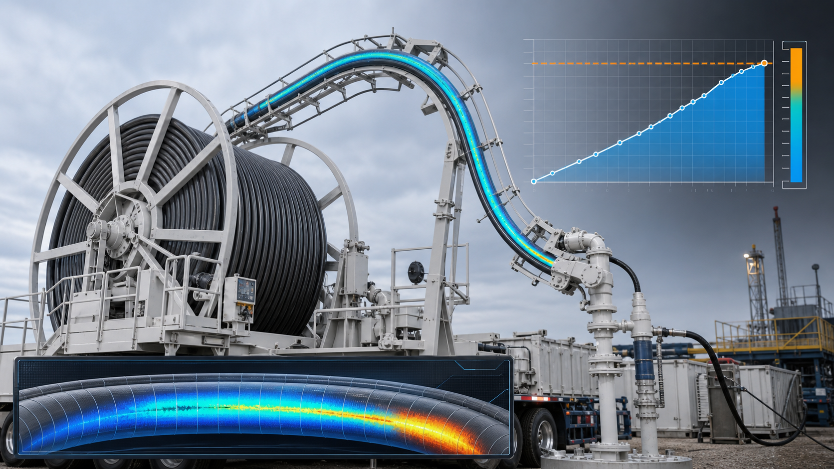
The chart below plots this curve for illustrative constants (sigma_f = 120, b = −0.12) — swap in your own vendor curve constants before using this on a real string. Read it left to right: fewer cycles to failure at high stress, many more at low stress. At N_f = 5,000 cycles, this curve reads a stress amplitude of about 39.7.

Step 2 — Log every job’s bend cycles
The curve is only useful if you feed it real numbers, job by job. For every job, record the bend cycles the string saw (roughly, trips in and out over the reel and gooseneck), the estimated stress amplitude for that job’s bend radius and pressure, and the resulting damage increment. Here’s a sample log for four recent jobs on one string:
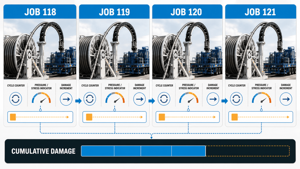
Notice the damage increment isn’t proportional to bend cycles alone — Job 119 ran fewer cycles than Job 118 but did more damage per cycle, because it ran at a tighter bend or higher pressure. That’s exactly why you need the curve, not a cycle count alone, to track fatigue correctly. A simpler tracker that just counted total bend cycles and compared them to a single flat life number would have cleared Job 119 without a second look — and quietly let a harder-on-the-pipe job pass for less than it actually cost the string.
Step 3 — Work one job by hand
Before you trust any script, work one job by hand so you know exactly what the automation should produce. Take Job 121 from the log above: 1,325 bend cycles, engineered stress amplitude sigma_a = 29.0 on our illustrative curve.
Step 3a — cycles to failure at this stress:
N_f = 0.5 × (29.0 / 120) ^ (1 / −0.12) = 0.5 × (0.2417) ^ (−8.333) ≈ 69,000 cycles
Step 3b — damage from this job:
ΔD = n / N_f = 1,325 / 69,000 ≈ 0.019
Step 3c — add it to the string’s running total. Say this string entered the week with 0.363 of cumulative damage from its service history. Add Jobs 118–121’s increments (0.011 + 0.014 + 0.013 + 0.019 = 0.057) and the string now sits at:
D = 0.363 + 0.057 = 0.42
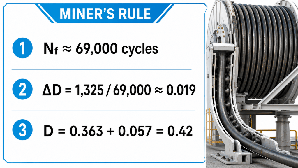
This is Miner’s Rule — cumulative damage is just the sum of each job’s fraction of the string’s fatigue life, D = Σ(n_i / N_i). Failure is predicted at D = 1.0, but most operators retire or inspect strings well before that, commonly in the 0.6–0.8 range, to keep a safety margin against the uncertainty baked into any fatigue curve.
Step 4 — Automate it in Python
Once you trust the hand calculation, turn it into a script that runs on every job’s data without anyone re-deriving it. This one reads a CSV job log, computes N_f and the damage increment for each row with pandas, and flags the string the moment it crosses your retirement threshold:
import pandas as pd# Fatigue curve constants -- replace with your vendor's engineering dataSIGMA_F = 120.0B = -0.12RETIREMENT_THRESHOLD = 0.60def cycles_to_failure(sigma_a, sigma_f=SIGMA_F, b=B): """Basquin's relation, solved for cycles to failure.""" return 0.5 * (sigma_a / sigma_f) ** (1 / b)def track_fatigue(job_log_csv, starting_damage=0.0): """ job_log_csv columns required: job_id, bend_cycles, stress_amplitude Returns the log with N_f, damage increment, and running cumulative damage per job. """ jobs = pd.read_csv(job_log_csv) jobs["N_f"] = cycles_to_failure(jobs["stress_amplitude"]) jobs["delta_D"] = jobs["bend_cycles"] / jobs["N_f"] jobs["cumulative_D"] = starting_damage + jobs["delta_D"].cumsum() jobs["retire_flag"] = jobs["cumulative_D"] >= RETIREMENT_THRESHOLD return jobsif __name__ == "__main__": log = track_fatigue("ct_job_log.csv", starting_damage=0.363) print(log[["job_id", "bend_cycles", "N_f", "delta_D", "cumulative_D", "retire_flag"]]) if log["retire_flag"].any(): flagged = log.loc[log["retire_flag"], "job_id"].iloc[0] print(f"RETIREMENT THRESHOLD CROSSED at job {flagged}")
Run it against Jobs 118–121 from Step 3 with starting_damage=0.363 and it reproduces the hand calculation exactly — cumulative damage of 0.42 after Job 121, well clear of a 0.60 threshold. Point it at a longer job history and it becomes a running tracker: plot cumulative_D against job number and you get a trend line that tells you, at a glance, how many jobs of headroom a string has left before it needs to come off the string count.

That chart came straight out of matplotlib plotting log["cumulative_D"] for a different string’s last twelve jobs — the same tracker function, just fed a longer CSV. Once the pipeline exists, adding a new job is a one-line append to a CSV instead of an afternoon in a spreadsheet.
Keep the script itself under version control alongside your curve constants, and treat any change to SIGMA_F, B, or RETIREMENT_THRESHOLD the same way you’d treat a change to a written procedure — with a reason logged and a second set of eyes. The arithmetic is easy to automate; the engineering judgment behind the constants isn’t, and that’s exactly the part that should still involve a person.
Expected result and how to check it
Your sanity check is the worked example itself: feed the tracker Jobs 118–121 with starting_damage=0.363 and it should land on cumulative_D = 0.42 after Job 121, matching Step 3 to two decimal places. If it doesn’t, check three things first — the sign on b (it must be negative), whether starting_damage got left at its default of zero, and whether your CSV’s stress_amplitude column is actually in the same index units as SIGMA_F.
- Don’t mix curve units. A stress amplitude computed against one vendor’s fatigue curve is meaningless plugged into another vendor’s
sigma_fandb. Keep the source of your curve constants documented next to the code. - Don’t drop the starting damage. A string doesn’t start its life the day you started tracking it in Python — carry forward whatever cumulative damage it already had from its BOL reset or last inspection, or every number downstream will read artificially low.
- Don’t treat D = 1.0 as your line in the sand. That’s the point the curve predicts failure, not the point you should still be running the string. Set
RETIREMENT_THRESHOLDto whatever conservative value your engineering standards call for, and let the script flag it early. - Don’t let the model run unchecked forever. Where you have real inspection data — a string pulled for wall-thickness testing, or one that actually failed — feed that back against what the tracker predicted at the time. A model that’s drifted from reality is worse than a spreadsheet nobody trusted in the first place, because it looks authoritative.
If you’re building out a broader automated toolkit around this string, our related tutorials on automating coiled tubing friction pressure calculations and converting nitrogen job volumes with a real-gas Z factor cover the other two calculations most CT job plans need before the string ever goes in the hole.
Download the Coiled Tubing Fatigue Life Studio
I have already done the heavy engineering and software work for you. Instead of rebuilding the tracker from this tutorial, you can download the EnergyMindAI CT Fatigue Life Studio v1.0.0: a professional, portable Windows application for maintaining a cumulative coiled tubing fatigue life history across multiple strings and jobs. It runs directly on Windows without installing Python or any third-party engineering package, and the first 30 days are free.
Windows 10/11 · No Python required · 30-day free trial · ZIP download: 43.1 MB
What does this coiled tubing fatigue life tool calculate?
The application divides the physical string into tracked segments and applies a transparent low-cycle-fatigue screening model. It combines plastic bending over the reel and gooseneck with thick-wall pressure stresses, applied axial load, weld penalties, wall loss, ovality and environmental severity. Incremental damage is accumulated with Miner’s Rule so every committed job updates the same string history rather than producing an isolated one-off answer.
- Import real job data: load CSV or ordinary XLSX files containing elapsed time, depth, pump pressure, wellhead pressure, axial force, speed, temperature and job notes.
- Enter data manually: add or edit operating points when a clean digital file is unavailable.
- Track multiple CT strings: save each string’s geometry, material inputs, starting fatigue profile, weld map and complete job history in a local engineering library.
- Model weld locations: identify bias welds, tapered bias welds, dressed or undressed butt welds and field welds with configurable life factors.
- Review stresses: inspect hoop, radial, axial, bending and von Mises stress results together with strain and incremental fatigue damage.
- Screen service environments: record acid, H2S, CO2, produced water and chloride exposure, plus purging, pig or dart displacement and nitrogen plug-off practices.
- See the likely hotspot: play the animated reel-gooseneck-well view and display fatigue, damage and stress profiles along the string.
- Forecast repeat runs: test pressure, depth and axial-load scenarios without altering the saved string, then estimate how many comparable runs remain before the 80% engineering hold point.
- Export an audit package: create PDF and Word reports, dashboard graphics, segment-level CSV results and a JSON project backup.
How to start your first coiled tubing fatigue life project
1. Download and launch the portable Windows app
Download the ZIP, extract the complete folder, and double-click EnergyMindAI-CT-Fatigue-Life-Studio.exe. Windows may show a SmartScreen notice because this independent engineering build is not code-signed; choose the additional information option only after confirming the file hash below. The tool stores its library under your Windows user profile, not on the EnergyMindAI website.
2. Create the string before importing a job
Open String Library, create a unique string ID, and enter length, outside diameter, wall thickness, yield strength and the reel and gooseneck radii. Add known weld positions and segment-condition corrections. If an approved historical fatigue profile already exists, import it as the baseline so the calculation starts from the string’s actual accumulated life.
3. Import, preview and sanity-check the job
Load Sample-Job-Data.csv first to understand the required layout, then import the field file or enter the points manually. Review units carefully: depth is in feet, pressures are in psi, axial load is in lbf and temperature is in °F. Select the applicable fluids, gas exposure and string-care controls. Run Preview and check the depth-pressure trace, stress profile, weld peaks and maximum incremental damage before committing anything.
4. Commit the job and preserve the audit trail
Commit only after the preview matches the job record. The application adds that job’s damage to the selected string, updates the coiled tubing fatigue life profile and records the event in the audit log. Export a project backup after each accepted job, then create a PDF or Word report for the engineering file. Use the Run-Life Simulator for planning; it forecasts scenarios without changing the committed history.
Verification, file integrity and engineering limits
The release was tested after packaging and again after extraction on Windows. Automated checks cover thick-wall stress boundary conditions, strain-life monotonicity, pressure sensitivity, local weld penalties, physical string sweep selection, cumulative job commits, environmental modifiers, non-mutating forecasts, the 80% status rule, CSV/XLSX import, persistent project history and PDF/Word/CSV exports.
ZIP SHA-256:C3F177FD9EDD36C538F94D49794E849E35C1317F95F08F9BC86859FAB93971E8
Important: this is a transparent engineering screening and record-keeping tool, not a replacement for an OEM-validated fatigue model, the CT manufacturer’s retirement criteria, inspection or NDE, corrosion assessment, sour-service qualification, or competent engineering review. Default strain-life and environmental coefficients must be calibrated against your approved material and service data before operational decisions are made. The 80% threshold is implemented as a conservative user-specified engineering hold point; a low calculated percentage does not prove a string is fit for service.
For the theory behind the workflow, work through the equations and numerical example in this tutorial before relying on the software. You can also explore the EnergyMindAI upstream engineering tutorials for more practical Python and automation workflows.
