Coiled Tubing Friction Pressure Calculation

By Saad Iqbal

It’s 2 a.m. on location and the CT supervisor just asked you for a revised pump schedule because the job depth changed by 1,500 ft. You flip open the coiled tubing (CT) hydraulics chart book, squint at a Moody diagram under a headlamp, and start interpolating between curves that were plotted for someone else’s tubing size. Fifteen minutes later you have a number you’re only 80% sure of, and the crew is waiting. This is the moment a coiled tubing friction pressure calculation should take fifteen seconds, not fifteen minutes — and it can, once you automate it.

This tutorial walks through the physics behind coiled tubing friction pressure, then automates the whole calculation in about 25 lines of Python using the Darcy-Weisbach equation and the Swamee-Jain friction factor correlation. By the end you’ll have a reusable function that takes pump rate, CT size, and fluid properties and returns velocity, Reynolds number, friction factor, and total friction pressure in one call — plus a chart you can hand straight to the company man.

Prerequisites

Python 3.9 or newer installed (or a free notebook environment — see the tools list below)
Basic comfort with functions and floating-point math in Python; no numerical libraries required for the core calculation
matplotlib installed only if you want to reproduce the pump-rate chart in Step 5 (pip install matplotlib)
Your CT string’s OD, wall thickness, and the job’s target pump rate and fluid density on hand
10 minutes, and a coffee

Why Manual Coiled Tubing Friction Pressure Lookups Fall Apart

Printed friction charts are built for a handful of standard CT sizes and one or two fluid types. The moment your job uses a slightly worn string, a different wall thickness, or a gelled fluid instead of plain water, you’re extrapolating by eye. Coiled tubing friction pressure is also nonlinear with rate — it roughly follows velocity squared in turbulent flow — so a chart built for 1.5 bbl/min gives you a bad estimate at 3.0 bbl/min. Coding the calculation once removes both problems: you get an exact answer for your exact string, at any rate, in seconds.

Step 1 — Understand the Physics: Darcy-Weisbach

Friction pressure drop in a pipe is governed by the Darcy-Weisbach equation:

Δp = f · (L/d) · (ρv² / 2)

where Δp is the pressure drop, f is the dimensionless Darcy friction factor, L is pipe length, d is the inner diameter, ρ is fluid density, and v is average fluid velocity. Every term except f is easy to pin down from the job design. The friction factor is the one variable that depends on flow regime, and that’s where most manual lookups go wrong. The schematic below shows how the pieces map onto an actual CT rig-up: pump unit, CT reel, injector head, and the wellbore flow path where the pressure drop actually accumulates.

Figure 1 — the friction pressure flow path from pump to target zone.

Step 2 — Get the Friction Factor Right: Swamee-Jain

For laminar flow (Reynolds number Re < 2,300), f = 64/Re — trivial. But CT jobs are almost always turbulent, and the classic Colebrook-White equation for turbulent f is implicit — it has to be solved by iteration, which is exactly what makes chart lookups tempting in the first place. The Swamee-Jain equation is an explicit approximation of Colebrook-White, accurate to within about 1-2% across the turbulent range, and it drops straight into a Python one-liner:

f = 0.25 / [log₁₀(ε/(3.7d) + 5.74/Re^0.9)]²

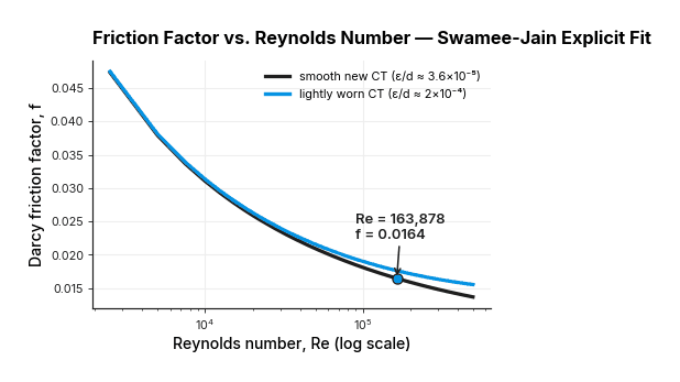
where ε is the pipe’s absolute roughness and Re = ρvd/μ is the Reynolds number. The chart below shows f falling as Re increases, for both a smooth new CT string and a lightly worn one — worth noting because a worn string can add several percent to your friction factor, and therefore your pump pressure, over the life of a reel.

Figure 2 — friction factor vs. Reynolds number, smooth vs. lightly worn CT.

Step 3 — Run the Worked Example

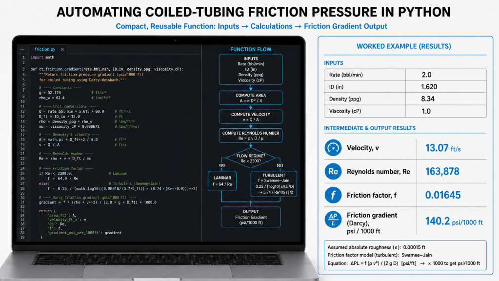
Let’s put real numbers through it. The job: 2″ OD × 0.190″ wall CT (1.62 in ID), pumping 8.34 ppg water-based fluid at 1.0 cP viscosity, at 2.0 bbl/min, down 10,000 ft of tubing. Converting rate to velocity through the CT’s cross-sectional area gives v = 13.07 ft/s (3.99 m/s) — well into turbulent flow. Reynolds number comes out to 163,878, the Swamee-Jain friction factor is 0.01645, and the resulting gradient is 0.1402 psi/ft, or 140.2 psi per 1,000 ft. Over the full 10,000 ft string, that’s 1,402 psi of friction pressure the pump has to overcome before it even starts working against hydrostatic and reservoir pressure downhole.

Figure 3 — inputs and results for the 2.0 bbl/min worked example.

Step 4 — Automate the Coiled Tubing Friction Pressure Calculation in Python

Here’s the whole calculation as a reusable function. It takes pump rate in bbl/min, CT inner diameter in inches, fluid density in ppg, and viscosity in cP, and returns velocity, Reynolds number, friction factor, and gradient in psi/1,000 ft:

			
import math
def swamee_jain_f(re, rel_rough):
    return 0.25 / (math.log10(
        rel_rough/3.7 + 5.74/re**0.9))**2
def friction_calc(rate_bbl_min, id_in, ppg, cp, rough_mm=0.0015):
    Q = rate_bbl_min * 0.158987 / 60      # m3/s
    d = id_in * 0.0254                    # m
    rho = ppg * 119.8264                  # kg/m3
    mu = cp * 0.001                       # Pa.s
    A = math.pi/4 * d**2
    v = Q / A
    re = rho * v * d / mu
    f = 64/re if re < 2300 else swamee_jain_f(
        re, (rough_mm/1000)/d)
    grad_pa_m = f * rho * v**2 / (2*d)
    return v/0.3048, re, f, grad_pa_m * 4.4211e-5
# 2" OD x 0.190" CT, water 8.34 ppg, 1 cP, 2.0 bbl/min
v, re, f, grad = friction_calc(2.0, 1.62, 8.34, 1.0)
print(f'v={v:.2f} ft/s   Re={re:,.0f}   f={f:.4f}   grad={grad*1000:.1f} psi/1000ft')
# -> v=13.07 ft/s   Re=163,878   f=0.0164   grad=140.2 psi/1000ft

		

Figure 4 — the friction_calc() function, matching the worked example exactly.

Multiply the returned gradient by (well depth in ft / 1,000) to get total friction pressure for any job length — that’s the number you add to hydrostatic and reservoir pressure to get required surface pump pressure. If you’re already tracking job parameters in a Python-based workflow, this same pattern of wrapping a real engineering correlation in a small function is the same approach we used for decline curves and nodal analysis — see the nodal analysis tools comparison if you want to take IPR/VLP modeling further with free Python plotting.

Step 5 — Chart It Across Rates for Job Planning

A single number is useful for right now; a curve is useful for planning the whole job. Loop friction_calc() across a range of pump rates for each CT size you might run, and you get a chart the crew can read off during rate changes instead of calling the office. The chart below covers three common CT IDs — 1.25 in, 1.62 in, and 1.995 in — from 0.5 to 4.0 bbl/min, with the 2.0 bbl/min worked example marked at 140.2 psi/1,000 ft.

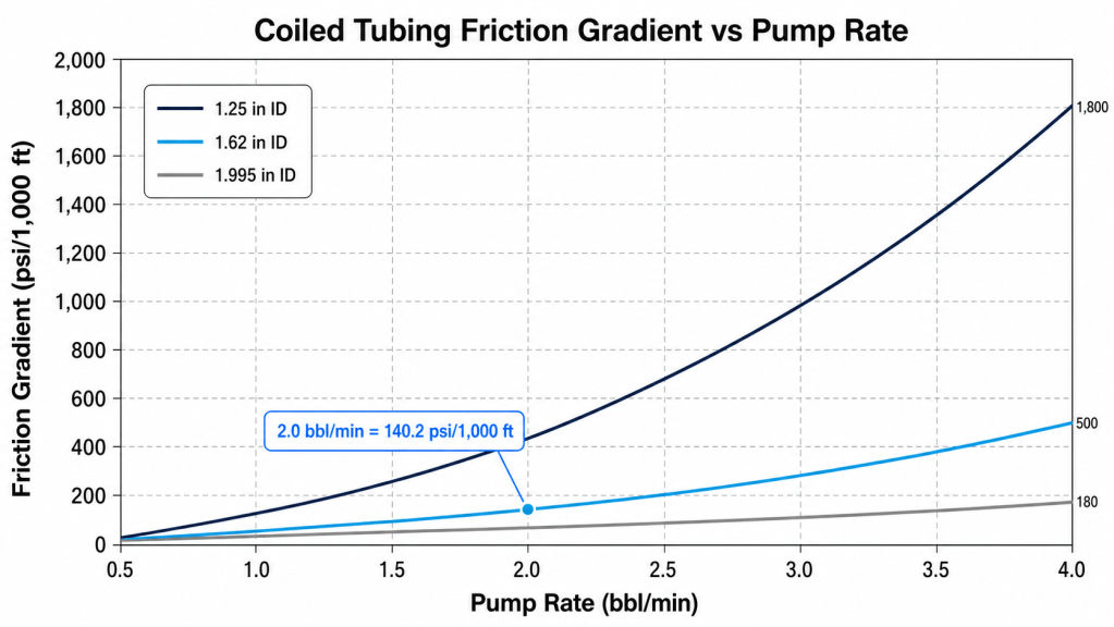
Figure 5 — friction gradient vs. pump rate for three CT diameters.

Notice how steeply the smaller 1.25 in ID string climbs compared to the 1.995 in string — at 4.0 bbl/min the small string is pushing nearly 1,800 psi/1,000 ft, almost ten times the large string’s gradient. That’s the kind of nonlinear behavior a single chart-book curve can’t show you across sizes, but a five-line loop can.

Verify Your Numbers and Common Pitfalls

Check the flow regime. Confirm Re > ~2,300 before using Swamee-Jain — below that, switch to f = 64/Re for laminar flow, or your friction factor will be wrong by an order of magnitude.
Roughness matters more than people think. New CT is very smooth (ε ≈ 0.0015 mm used here); a worn or corroded string can be several times rougher. If your friction pressure keeps reading low against actual surface pressure, bump the roughness input up and see if the model tracks the difference.
Watch your units. The most common bug in a hand-rolled version of this function is mixing psi with Pa or ppg with kg/m³ mid-formula. Keep the unit conversions inside the function, as shown, so every call is consistent.
Cross-check against a second source. Before you trust this on a live job, run the same inputs through an independent calculator — see the tools below — and confirm the two agree within a percent or two.
This is friction pressure only. Total required surface pressure still needs hydrostatic pressure, any reservoir/backpressure term, and CT-specific effects like helical buckling or reel friction added on top — this function solves one piece of the puzzle, not the whole pump schedule.

Tools Referenced in This Tutorial

Python — the free, open-source language used for every calculation in this tutorial.
Engineers Edge Swamee-Jain Friction Factor Calculator — a free online calculator to independently cross-check your f and Re values.
NOV Coiled Tubing Calculator — an industry hydraulics/pressures tool built specifically around CT string sizes, useful for a second-opinion sanity check on a live job.

Once this function lives in your job-planning scripts, the 2 a.m. depth-change request stops being a fifteen-minute chart-flipping exercise and becomes a fifteen-second function call — and every rate on the pump schedule gets the same rigor as the first one. If you’re building out a broader upstream automation toolkit, our tutorial on automating pipeline corrosion calculations follows the same pattern for a completely different well-integrity problem.