

By Saad Iqbal
A production engineer building an IPR for a new well has oil gravity, a solution gas-oil ratio from the DST, and a reservoir temperature off the log header — and nothing else. The full PVT lab report is three weeks out, but the nodal analysis model is due Friday, and the tubing performance curve can’t be built without a viscosity value at reservoir pressure and temperature. Guessing a round number like “2 cp” is how a perfectly good well gets modeled as a marginal one, or vice versa — oil viscosity is one of the biggest levers on both inflow performance and frictional pressure drop in the tubing string.
Correlations exist for exactly this situation, and they’re accurate enough to build a defensible early model: Beggs and Robinson for dead (gas-free) oil viscosity, and Chew and Connally to add the effect of dissolved gas once the oil is live. This tutorial runs both, then extends the result above the bubble point, and automates the whole chain in Python.
Prerequisites
- Stock-tank oil gravity, °API — here, 35° API.
- Reservoir temperature, T — here, 150°F.
- Solution gas-oil ratio at the pressure of interest, Rs (scf/STB) — here, 500 scf/STB at the bubble point.
- Bubble-point pressure, pb, and the reservoir (or flowing) pressure, p, if that pressure is above the bubble point — here, pb = 2,500 psi and p = 3,500 psi.
- Python 3 with
numpyinstalled (pip install numpy), or a spreadsheet.
Step 1 — Dead-Oil Viscosity with Beggs-Robinson
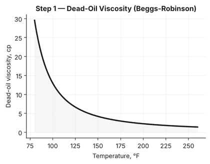
Dead-oil viscosity is the gas-free baseline every other PVT viscosity correlation builds from. The Beggs-Robinson (1975) correlation needs only API gravity and temperature:
Z = 3.0324 − 0.02023 × APIY = 10^ZX = Y × T^(−1.163) (T in °F)μoD = 10^X − 1 (cp)
Working the 35° API, 150°F case through it: Z = 3.0324 − 0.02023(35) = 2.324, so Y = 10^2.324 = 211.1. Then X = 211.1 × 150^(−1.163) = 211.1 × 0.002946 = 0.622, and μoD = 10^0.622 − 1 = 3.19 cp.
That 3.19 cp is the gas-free viscosity — before any solution gas is accounted for. For reference, the same oil at 100°F comes out to 8.91 cp, and at 200°F it drops to 1.78 cp: dead-oil viscosity is steeply temperature-dependent, which is exactly why a correlation built on both API and T, rather than API alone, is worth using.

Step 2 — Live-Oil (Saturated) Viscosity with Chew-Connally
Dissolved gas lowers viscosity substantially — an oil that’s 3.19 cp dead can easily be under 1.5 cp once gas is in solution. The Chew-Connally (1959) correlation applies that reduction as a function of Rs:
A = 10^[Rs × (2.2×10⁻⁷ × Rs − 7.4×10⁻⁴)]b = 0.68/10^(8.62×10⁻⁵×Rs) + 0.25/10^(1.10×10⁻³×Rs) + 0.062/10^(3.74×10⁻³×Rs)μob = A × μoD^b
At Rs = 500 scf/STB: A = 10^[500×(2.2×10⁻⁷×500 − 7.4×10⁻⁴)] = 10^(−0.315) = 0.484. The exponent b works out to 0.616 + 0.070 + 0.001 = 0.687. So μob = 0.484 × 3.19^0.687 = 0.484 × 2.219 = 1.07 cp — less than a third of the dead-oil value, which is the normal order of magnitude for gas-cut reduction at this Rs.
Running the same oil at Rs = 200 scf/STB gives μob = 1.87 cp, and at Rs = 800 scf/STB it drops further to 0.72 cp — more dissolved gas keeps pushing the viscosity down, which is why a well’s produced-fluid viscosity falls as flowing bottomhole pressure drops toward the bubble point.

Step 3 — Above the Bubble Point: the Undersaturated Correction
Everything above applies at or below the bubble point, where Rs still changes with pressure. Above pb, no more gas goes into solution, so Rs is fixed — but rising pressure still compresses the liquid slightly and raises viscosity a little. The Vasquez-Beggs undersaturated correction captures that:
m = 2.6 × p^1.187 × 10^(−3.9×10⁻⁵×p − 5)μo = μob × (p / pb)^m
With pb = 2,500 psi and a reservoir pressure p = 3,500 psi: m = 2.6 × 3500^1.187 × 10^(−3.9×10⁻⁵×3500 − 5) = 2.6 × 16,166 × 7.31×10⁻⁶ = 0.307. Then μo = 1.07 × (3500/2500)^0.307 = 1.07 × 1.11 = 1.19 cp at reservoir pressure — a modest rise from the 1.07 cp bubble-point value, which is the expected magnitude for a 1,000 psi overpressure above pb.
That three-stage chain — dead oil, saturated live oil, undersaturated correction — is exactly what a PVT correlation module needs to hand off a usable viscosity to an IPR or nodal analysis model at any pressure in the well’s operating range.
Automating the Chain in Python
Once the three formulas are in hand, wrapping them into one function that takes pressure as the only variable (holding API, T, and the Rs-vs-pressure behavior fixed) makes it trivial to generate a full viscosity-vs-pressure curve for a tubing performance calculation:
import numpy as np

def dead_oil_viscosity(api, temp_f):
    Z = 3.0324 - 0.02023 * api
    Y = 10 ** Z
    X = Y * temp_f ** (-1.163)
    return 10 ** X - 1  # cp

def live_oil_viscosity(mu_dead, rs):
    A = 10 ** (rs * (2.2e-7 * rs - 7.4e-4))
    b = (0.68 / 10 ** (8.62e-5 * rs)
         + 0.25 / 10 ** (1.10e-3 * rs)
         + 0.062 / 10 ** (3.74e-3 * rs))
    return A * mu_dead ** b  # cp

def undersaturated_viscosity(mu_bubble, p, pb):
    m = 2.6 * p ** 1.187 * 10 ** (-3.9e-5 * p - 5)
    return mu_bubble * (p / pb) ** m  # cp

api, temp_f, rs, pb, p = 35, 150, 500, 2500, 3500

mu_dead = dead_oil_viscosity(api, temp_f)
mu_bubble = live_oil_viscosity(mu_dead, rs)
mu_reservoir = undersaturated_viscosity(mu_bubble, p, pb)

print(f"Dead oil:        {mu_dead:.2f} cp")
print(f"At bubble point: {mu_bubble:.2f} cp")
print(f"At {p} psi:      {mu_reservoir:.2f} cp")
# Dead oil:        3.19 cp
# At bubble point: 1.07 cp
# At 3500 psi:     1.19 cp
Loop that over a pressure array from the bubble point up to the maximum reservoir pressure (using the undersaturated branch) and down to atmospheric (recomputing Rs from a solution-gas correlation like Standing’s at each pressure step below pb), and you have a full viscosity-vs-pressure table ready to feed straight into an inflow performance or multiphase-flow calculation.
Verification and Pitfalls
Check any correlation result against a sanity range before trusting it in a model: dead-oil viscosity for a 30–40° API crude at typical reservoir temperatures should generally fall somewhere between 1 and 15 cp, and live-oil viscosity should always come out lower than the dead-oil value at the same temperature — if it doesn’t, check that Rs and the dead-oil viscosity were computed at consistent conditions. Where a real PVT lab report is available, always prefer the lab-measured viscosity over the correlation; these correlations exist to bridge the gap before lab data exists, or to sanity-check a lab result that looks suspicious.
The most common mistake is applying Chew-Connally with an Rs value that doesn’t match the pressure being evaluated — Rs has to come from the correct point on the solution-gas-vs-pressure curve for that same pressure, not the bubble-point Rs used indiscriminately at every pressure below pb. A second common error is forgetting the undersaturated branch entirely and using the bubble-point viscosity for every pressure above pb, which quietly under-predicts viscosity (and therefore under-predicts frictional pressure drop) at higher flowing pressures. Finally, both Beggs-Robinson and Chew-Connally were developed on specific crude-oil datasets; for very heavy oil (under 20° API) or very light, highly volatile oil, their error grows, and a lab measurement or a more specialized correlation is worth the wait.
For the companion correlation that gets you Rs and bubble-point pressure in the first place, see Standing’s Correlation: Bubble Point Pressure and Oil FVF. And once viscosity is in hand, it plugs directly into the kind of continuously-updated well model described in AI Nodal Analysis Software for Production Optimization.
