Productivity Index and Skin Factor: Step-by-Step Calculation

By Saad Iqbal

Two wells with identical reservoir rock can produce very differently, and the reason is usually written in two numbers: productivity index and skin factor. Productivity index (J) tells you how many barrels per day you get for every psi of drawdown; skin factor (s) tells you how much of your well’s potential is being lost to near-wellbore damage. This tutorial works through both—by hand and in Python—so you can diagnose an underperforming well instead of just watching its decline curve.

Prerequisites

• Effective permeability, k (millidarcies)
• Net pay thickness, h (ft)
• Oil viscosity, μ_o (cp), and formation volume factor, B_o (rb/stb)
• Drainage radius, r_e, and wellbore radius, r_w (ft)
• An estimate of skin factor, s, from a pressure transient (build-up/draw-down) test
• Python 3 with pandas for tracking J over time as skin changes

The physical picture behind the math is radial flow converging from the drainage boundary down to the wellbore—skin factor is effectively an extra, localized resistance right at that final step:

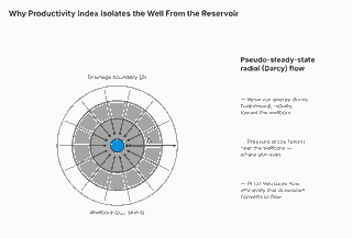
The formula

For a well in pseudo-steady-state radial flow, the productivity index is:

where J is in stb/day/psi, k is permeability in md, h is net pay in ft, μ_o is oil viscosity in cp, B_o is the formation volume factor in rb/stb, r_e and r_w are drainage and wellbore radii in ft, and s is the dimensionless skin factor (zero for an undamaged well, positive for damage, negative for a stimulated well).

Worked example

Take a well with k = 50 md, h = 30 ft, μ_o = 1.5 cp, B_o = 1.25 rb/stb, r_e = 1,000 ft, r_w = 0.33 ft, and a build-up test indicating s = 5 (moderate near-wellbore damage):

import math
k = 50       # md
h = 30       # ft
mu_o = 1.5   # cp
Bo = 1.25    # rb/stb
re = 1000    # ft
rw = 0.33    # ft
s = 5        # skin factor from build-up test
ln_term = math.log(re / rw)
J = 0.00708 * k * h / (mu_o * Bo * (ln_term - 0.75 + s))
print(round(J, 3), "stb/day/psi")
# -> 0.462 stb/day/psi
# compare against an undamaged well (s = 0)
J_ideal = 0.00708 * k * h / (mu_o * Bo * (ln_term - 0.75))
print("PI lost to skin:", round((1 - J / J_ideal) * 100, 1), "%")
# -> 40.8 percent of potential productivity lost to damage

At J = 0.462 stb/day/psi, this well is producing at barely 59% of what an undamaged completion would deliver with the same reservoir properties—a strong economic case for a stimulation treatment or acid wash.

Automating it with Python and pandas

Skin factor isn’t static—it drifts with scale buildup, fines migration, and workovers. Tracking J alongside periodic skin estimates lets you catch degradation (or confirm a successful stimulation) before it shows up as a surprise in the production report:

import pandas as pd
import numpy as np
def productivity_index(k, h, mu_o, Bo, re, rw, s):
    """Vectorized productivity index (stb/day/psi)."""
    ln_term = np.log(re / rw)
    return 0.00708 * k * h / (mu_o * Bo * (ln_term - 0.75 + s))
# periodic well-test history: one row per build-up/draw-down survey
df = pd.DataFrame({
    "test_date": pd.date_range("2026-01-01", periods=8, freq="MS"),
    "k_md": 50,
    "h_ft": 30,
    "mu_o_cp": 1.5,
    "Bo_rb_stb": 1.25,
    "re_ft": 1000,
    "rw_ft": 0.33,
    "skin": [2, 2.5, 3.2, 4.0, 5.0, 4.6, 3.1, 2.0],  # rises then drops after stimulation
})
df["J_stb_day_psi"] = productivity_index(
    df["k_md"], df["h_ft"], df["mu_o_cp"], df["Bo_rb_stb"],
    df["re_ft"], df["rw_ft"], df["skin"]
)
print(df[["test_date", "skin", "J_stb_day_psi"]])

Monitoring the trend

Plotted over time, a well with worsening formation damage shows J declining as skin climbs, then recovering sharply after a successful intervention—exactly the signature you want your production-surveillance dashboard to flag automatically:

Tools used

• Python 3 with pandas and NumPy for batch calculation across a well test history
• Jupyter Notebook for interactive build-up test analysis
• Power BI or Looker Studio for dashboarding PI trends across a field
• Claude or ChatGPT for interpreting ambiguous build-up test shapes before committing to a skin estimate

Verifying your result

Cross-check J against the well’s actual test rate divided by its observed drawdown (q/Δp)—they should be in the same ballpark if your input parameters are representative of current reservoir conditions. A skin factor that comes out strongly negative (below about −5) usually points to a successfully stimulated or naturally fractured well; a value above 10–15 suggests severe damage worth investigating before you trust the number blindly.

Common pitfalls

• Mixing up r_e and the wellbore radius. These differ by orders of magnitude; a transposed value silently produces a nonsensical J.
• Treating skin as permanent. Skin changes with scale, fines, and workovers—re-run build-up tests periodically rather than relying on a value from years ago.
• Ignoring units on k and h. The 0.00708 constant is calibrated for md, ft, cp, and rb/stb specifically—swap in SI units without converting the constant and the result will be off by orders of magnitude.

Related reading

• Nodal Analysis for an Oil Well: IPR Meets VLP — where productivity index feeds into a full well-performance model
• Vogel IPR Equation: Calculate AOF and the IPR Curve — the inflow relationship for solution-gas-drive reservoirs below bubble point
• ESP TDH Calculation — sizing artificial lift once you know what the well can actually deliver
• Sucker Rod Pump Volumetric Efficiency — another lift-side diagnostic worth pairing with a PI trend

Want to track this across your whole field? Extend the pandas snippet above with one row per well per test date, then feed the output straight into your production-surveillance dashboard.