
By Saad Iqbal
An engineer staring at a wellhead readout doesn’t actually know, in real time, how much steel is left in the tubing wall. What he has is a corrosion coupon pulled during the last workover, or an inline inspection (ILI) run stamped with a date from ten months ago. Both are snapshots. Neither one tells him what happened last Tuesday, when water cut climbed, the inhibitor pump lost prime for six hours, and the flowline briefly ran hotter and faster than design ever assumed. By the time the next report lands, the well could already be weeks past a safe reinspection interval — or, in a sour system, quietly building toward a sulfide-stress-cracking failure nobody saw coming.
This is the gap that AI corrosion rate prediction for oil and gas wells is starting to close. Instead of treating corrosion as something you measure occasionally and infer the rest of the time, machine learning models fed by real-time sensors turn wall loss into a continuous number — one that updates every shift, not every annual pigging campaign. It’s less a new instrument than a new habit of mind: corrosion stops being a report you wait for and becomes a signal you watch.
Why CO2 and H2S Corrosion Are the Real Threat to Upstream Tubulars
Produced fluids in most oil and gas wells carry dissolved CO2, and a meaningful share also carry H2S. Both attack carbon steel, but they don’t attack it the same way, and conflating them is where a lot of integrity programs get into trouble.
“Sweet” corrosion — CO2 in produced water forming carbonic acid — is primarily a wall-loss problem. It thins tubing, casing and flowlines steadily, and that thinning eats directly into remaining life: the pressure and collapse ratings an engineer relies on were calculated for a nominal wall thickness, and every fraction of a millimeter of loss quietly derates the pipe underneath the number on the tally book. This is the same underlying wall-loss logic covered in our piece on AI casing wear prediction — a different mechanical cause, but the same consequence: a string that looks fine on paper until someone actually measures it.
“Sour” corrosion — H2S in the system — is a different animal. Beyond general wall loss, dissolved H2S can drive sulfide stress cracking (SSC), hydrogen-induced cracking (HIC) and stress-oriented hydrogen-induced cracking (SOHIC): brittle, sometimes sudden failure modes that a corrosion coupon measuring average metal loss is poorly equipped to catch. That’s exactly why sour service is governed by its own standard, NACE MR0175 / ISO 15156, which sets material hardness limits, metallurgy and heat-treatment requirements specifically to keep steel resistant to cracking once H2S partial pressure and pH put a system into “sour” territory. A well can post a perfectly reassuring coupon result and still be running metallurgy that isn’t appropriate for how sour it has actually become.
What Actually Drives a Well’s CO2 Corrosion Rate?
Long before machine learning entered the picture, corrosion engineers had a trusted physical baseline: the de Waard-Milliams model, first published in 1975 and refined over the years — notably by de Waard, Lotz and Dugstad — into what’s often called the de Waard-Lotz-Dugstad correlation. In parallel, the Norwegian NORSOK M-506 standard built its own CO2 corrosion rate calculation model on similar physics, adding corrections for wall shear stress, bicarbonate buffering and glycol content that make it better suited to real multiphase flowlines rather than idealized lab conditions. Both are still the reference points an experienced engineer checks a new prediction against.
The governing relationship, at a conceptual level, comes down to four drivers:
- CO2 partial pressure (fugacity): more dissolved CO2 means more carbonic acid in the water phase, and higher partial pressure pushes the uninhibited corrosion rate up.
- Temperature: corrosion rate rises with temperature, because the reaction kinetics simply run faster — but only up to a point, roughly the 60–80°C range. Past that, an adherent iron carbonate (siderite) scale tends to form and stick to the steel, and that protective layer can pull the corrosion rate back down even though the temperature is higher. This is the well-known “hump” shape in the de Waard-Milliams curve, and it’s the single most common place engineers get the relationship backwards.
- pH: lower pH means more aggressive water chemistry and a faster rate; anything that buffers pH upward — bicarbonate, a scale layer, treatment chemistry — works against corrosion.
- Flow velocity and wall shear stress: this is what decides whether that protective siderite scale actually gets to do its job. At low shear, scale can form and stay put. At high shear — a fast flowline, a choke, a bend — the same scale can be mechanically stripped off, exposing fresh steel and pushing the effective corrosion rate back up even in a temperature range that should otherwise be self-limiting.
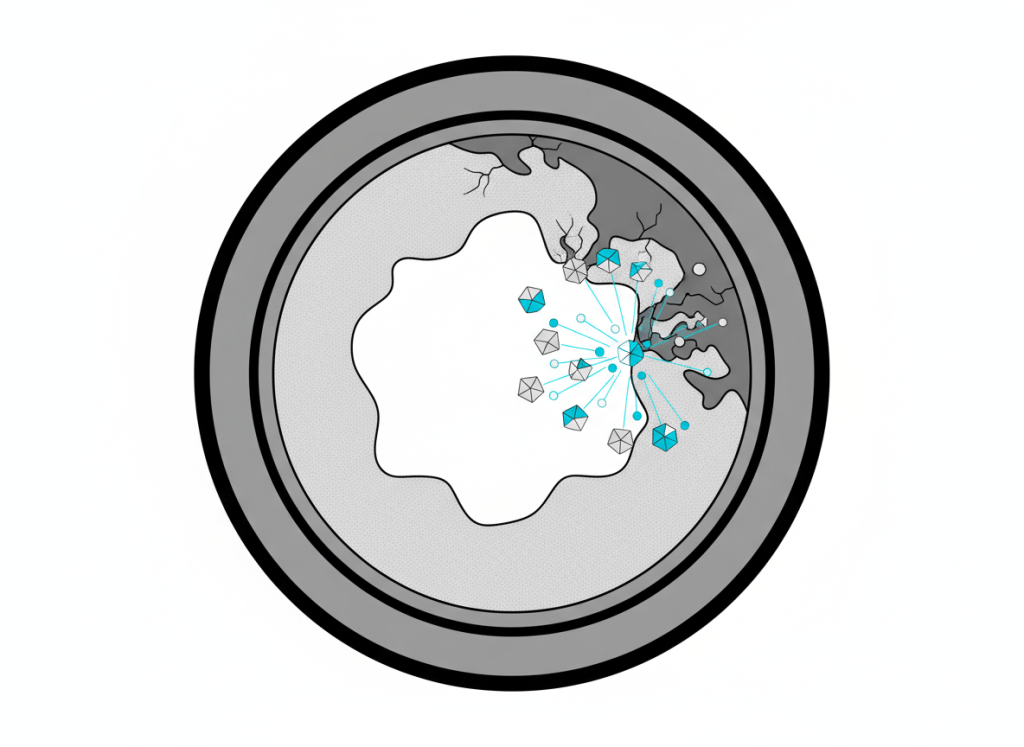
To make this concrete: at roughly 1 bar of CO2 partial pressure and 20°C, an uninhibited de Waard-Milliams-style estimate typically lands somewhere in the rough neighborhood of 1–2 mm/year. Hold that same CO2 partial pressure and raise the temperature toward 60–70°C, and the uninhibited estimate can climb toward 3–5 mm/year. Push further, into a regime where a stable siderite film forms and adheres, and the same CO2 partial pressure can show a markedly lower effective rate despite the higher temperature. Treat these as illustrative orders of magnitude, not a substitute for running NORSOK M-506 or a properly calibrated model against your own produced-water chemistry, inhibitor performance and flow regime.
How AI Corrosion Rate Prediction Works for Oil and Gas Wells
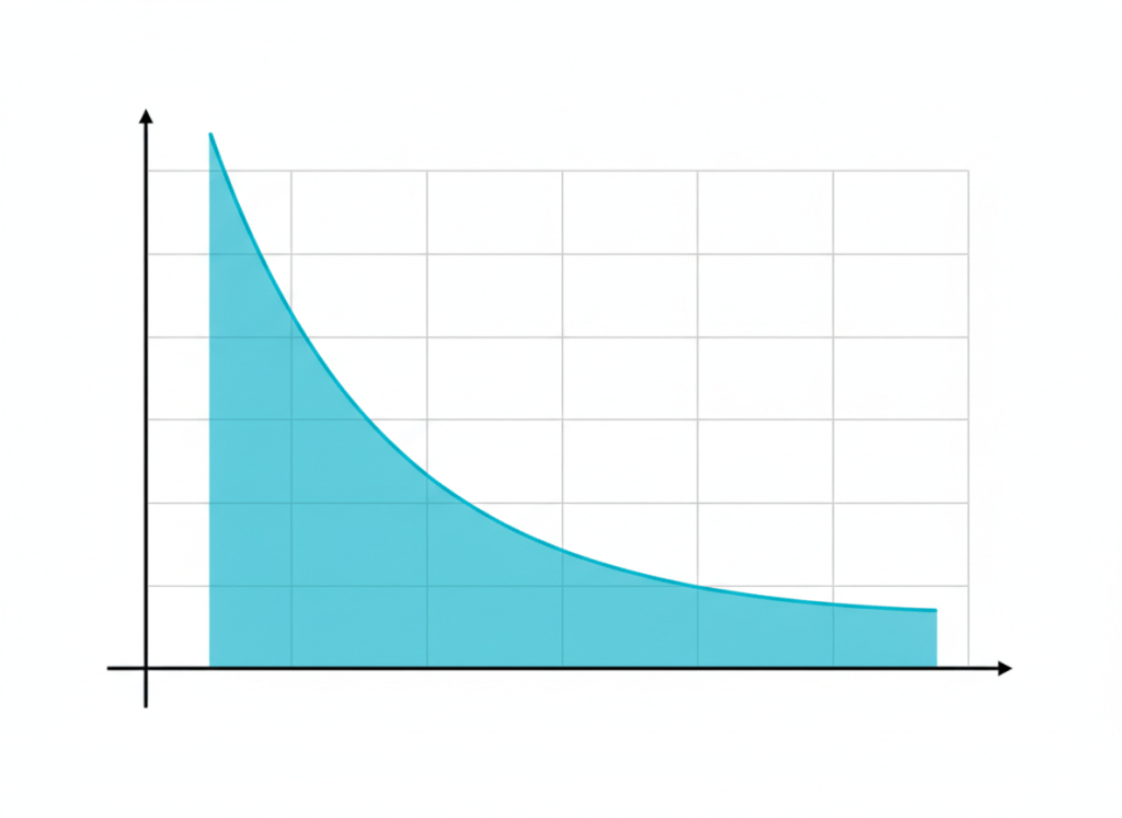
De Waard-Milliams and NORSOK M-506 give you a physics-based starting point. What they can’t easily do is absorb, minute by minute, everything actually happening downhole and in the flowline — and that’s the layer AI corrosion rate prediction adds.
The sensing layer is usually built on two familiar instruments. Electrical resistance (ER) probes measure metal loss directly, as a change in the electrical resistance of a thin sacrificial element exposed to the same fluid as the pipe wall. Linear polarization resistance (LPR) probes estimate instantaneous corrosion rate from the resistance to a small applied polarization, giving a faster-responding but noisier signal. Neither is new. What’s new is treating their continuous output as a live model input rather than a number an engineer glances at during a site visit.

A machine learning model built for this job typically ingests:
- Real-time ER and LPR probe readings from wellheads, manifolds and flowline monitoring stations.
- Process variables that drive the de Waard/NORSOK physics — CO2 partial pressure, temperature, pH, water cut and flow velocity — pulled from the process historian.
- Historical corrosion coupon results and prior ILI runs, used as ground truth to calibrate the model’s predictions against what physical inspection actually found.
- Inhibitor dosing and treatment history, since effective chemical treatment is itself one of the biggest levers on the observed rate.
Trained against that data, the model does three things a periodic report can’t: it produces a continuously updated corrosion rate and remaining wall life estimate per well or flowline segment; it flags anomalous acceleration — an inhibitor pump failure, a souring event, a flow regime change — days or weeks before it would show up in the next scheduled coupon pull; and it ranks wells and flowlines by urgency, so a limited inspection and treatment budget goes to the assets actually accelerating rather than being spread evenly across the portfolio on a fixed calendar. It’s the same underlying idea we covered in AI scale prediction for production wells — a different failure mechanism, the same shift from periodic inspection to continuous, model-driven monitoring.
Which Tools Actually Support This Workflow Today?
None of this requires exotic software. Most teams building an AI corrosion rate prediction pipeline are stitching together a fairly ordinary data-and-analytics stack:
- Python and pandas for the data pipeline — pulling ER/LPR telemetry, historian tags and lab coupon results into one modeling-ready dataset.
- Microsoft Power BI or Google Looker Studio for the monitoring dashboard operations actually watches day to day — remaining wall life by well, ranked by urgency.
- Cosasco, a long-established corrosion monitoring instrumentation supplier, on the sensing side — ER and LPR probes are exactly the hardware category feeding these models real data.
- Honeywell Forge’s Predict Corrosion Suite and Baker Hughes’ corrosion management offerings, as examples of vendor platforms built specifically to turn this kind of sensor and process data into predictive corrosion analytics at operator scale.

What This Changes for a Working Engineer’s Inspection Cadence
The practical shift isn’t that inspection stops mattering — it’s that inspection stops being purely calendar-driven. Instead of every well getting the same annual ILI run and the same coupon-pull schedule regardless of how it’s actually behaving, the wells and flowlines the model flags as accelerating move up the queue, and the ones running quietly stable can safely wait. Inhibitor dosing shifts the same way: from a fixed treatment schedule to adjustments triggered by an actual detected change in corrosion rate, rather than a response to a coupon result that’s already three months old.
That’s a meaningful change in how an integrity budget gets spent — fewer inspections wasted on wells that didn’t need them, and earlier warning on the ones that did.
Where AI Corrosion Rate Prediction Still Has Limits
None of this makes the model infallible, and a good engineer treats it accordingly.
- It needs real ground truth to learn from. A model calibrated against years of coupon and ILI history on a mature field is in a very different position than one deployed on a new asset with little inspection data to check itself against.
- Sensor drift and fouling are real failure modes of their own. ER and LPR probes can foul, drift, or simply measure a local condition that isn’t representative of the whole flowline — feed the model bad sensor data and it will confidently predict the wrong thing.
- It augments, it doesn’t replace, code-mandated inspection. Regulatory and code-driven ILI runs, hydrotests and inspection intervals still apply regardless of what the model says. The AI layer is a prioritization and early-warning tool sitting on top of that mandated baseline, not a substitute for it.
Used that way, AI corrosion rate prediction doesn’t replace the coupon or the ILI report — it fills the months of silence between them with an actual signal, so the next scheduled inspection confirms what the model already told you, rather than being the first time anyone found out.
If corrosion is only one piece of the integrity picture you’re trying to automate, our roundup of the best AI well integrity monitoring tools for 2026 is a good next stop for seeing how corrosion, casing wear and scale prediction fit into a single monitoring strategy.
