

By Saad Iqbal
Pull the caliper log on a well that just came off a hard, doglegged interval, and there’s a specific kind of dread that settles in. Somewhere in that build section, the casing wall has been quietly getting thinner every single hour the string rotated against it — and you find out about it days after the fact, from a wireline run, when the only options left are re-run, remediate, or gamble on the next completion. Casing wear prediction is how you stop finding out too late: instead of waiting for the caliper log, you calculate — and now increasingly let AI continuously calculate — exactly how much wall thickness a dogleg is going to eat before the bit ever gets there.
This is one of those problems that upstream drilling teams have quantified for decades but rarely tracked in real time. The math is well established. What’s changed is that automation now lets you run it continuously against live surface data instead of once, after the well, when it’s too late to do anything but react.
What Is Casing Wear Prediction, and Why Should It Matter to You?
Casing wear prediction is the practice of calculating, ahead of or during drilling, how much steel a rotating drill string will remove from the inside of a casing string through mechanical contact — mostly at tool joints, mostly in doglegs, build sections, and laterals where side force concentrates. It matters for three very practical reasons: a casing string that’s been worn thin fails its burst and collapse checks earlier than its design life assumed; a badly worn interval can force an operator into a remedial cement job or a liner they didn’t budget for; and in multi-well pad drilling, the same offset casing can get re-exposed to wear from every subsequent well drilled through it.
None of this is new to drilling engineers — casing wear factors have been part of torque-and-drag modeling since White and Dawson’s original work in the 1980s. What is new is treating the wear factor calculation as a live, continuously updated number instead of a single static check run once at the well-planning stage.
The Physics Behind Casing Wear Prediction
The model that underpins almost every casing wear prediction tool on the market — including commercial packages like Pegasus Vertex’s CWPRO — traces back to the same governing relationship: worn volume is proportional to the side (contact) force at the tool joint, the sliding distance, and a dimensionless wear factor that captures everything about mud type, tool-joint hardfacing, and casing metallurgy that isn’t explicitly modeled.
Written out, the volume of steel removed per foot of casing is:
WV = WF × SFdp × π × Dtj × 60 × N × t
- WV — worn volume, in³ per foot of casing
- WF — casing wear factor, expressed ×10⁻¹⁰ psi⁻¹ (typically 3–20 for water-based mud systems)
- SFdp — side force on the drill pipe at the contact point, lbf per foot
- Dtj — tool joint outer diameter, inches
- N — rotary speed, rpm
- t — total rotating time at that contact point, hours
The side force itself comes straight out of your torque-and-drag model — it’s highest exactly where you’d expect: at the low side of a build section, through doglegs, and anywhere the string is forced against the wall by curvature or buckling. If you’re already running torque-and-drag software, you already have the input this formula needs; casing wear prediction is really just one more output of the same model, not a separate discipline.

A Worked Example: Casing Wear Prediction Through a Real Dogleg
Take a build section generating 400 lbf/ft of side force on the drill pipe, a 5-inch tool joint OD, rotating at 120 rpm. Run the calculation for three wear factors — a well-inhibited water-based mud (WF = 5), a typical unweighted system (WF = 10), and an aggressive, poorly inhibited system (WF = 17) — and let rotating time in that interval climb from zero to 150 hours.
At WF = 10 and 40 hours of rotating time in the dogleg: WV = (10 × 10⁻¹⁰) × 400 × π × 5 × 60 × 120 × 40 ≈ 1.81 in³ per foot. Push the same interval to 78 hours and you cross roughly 6 in³/ft — a threshold worth flagging for a caliper run or a wear-factor recalibration, in this example. The high wear factor case reaches that same 6 in³/ft threshold in under half the rotating time.

Nothing about that math is exotic. What’s changed is who’s doing the arithmetic and how often. Run it by hand once at the planning stage and it’s a snapshot. Run it continuously against live rotary speed, hookload-derived side force, and elapsed rotating time, and it becomes a genuine early-warning system.
How AI Turns a Point Check Into Continuous Casing Wear Prediction
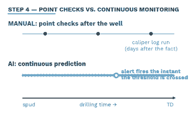
The manual version of this workflow looks the same at almost every operator: someone runs a torque-and-drag model before spud, picks a representative wear factor from experience or offset data, and checks the worst dogleg once. Then the well gets drilled, and the only way to know whether that estimate held up is a caliper log — days later, after the fact.
AI-assisted casing wear prediction — the same approach used in real-time drilling-engineering platforms and torque-and-drag software with live-data hooks — replaces that single check with a continuously updating one. Rotary speed, WOB-derived side force, and elapsed rotating time stream in from the rig’s data acquisition system every few seconds; the wear-volume model re-runs automatically; and the moment cumulative wear in any interval crosses your threshold, the directional driller or drilling engineer gets an alert while there’s still time to change mud properties, adjust rotary speed, or plan a wiper trip — not after the well is already down.
Automating the Casing Wear Formula With Python
You don’t need a commercial platform to stop doing this by hand — the White & Dawson relationship is a five-line function. Here’s the same worked example above, implemented so you can drop live rig-feed values in and get an alert instead of a static number:
import math

def casing_wear_volume(wear_factor, side_force_lbf_per_ft, tool_joint_od_in,
                        rotary_speed_rpm, rotating_hours):
    """
    White & Dawson casing wear volume model.
    wear_factor          : dimensionless casing wear factor (x1e-10 psi^-1), typically 3-20
    side_force_lbf_per_ft: contact/side force on the drill pipe, lbf/ft
    tool_joint_od_in     : tool joint outer diameter, inches
    rotary_speed_rpm     : rotary speed, rpm
    rotating_hours       : rotating time at this contact point, hours
    Returns worn volume in cubic inches per foot of casing.
    """
    wf = wear_factor * 1e-10
    return wf * side_force_lbf_per_ft * math.pi * tool_joint_od_in * 60 * rotary_speed_rpm * rotating_hours

# Worked example: medium wear factor, 400 lbf/ft side force, 5" tool joint, 120 rpm, 40 hours
wv = casing_wear_volume(wear_factor=10, side_force_lbf_per_ft=400,
                         tool_joint_od_in=5, rotary_speed_rpm=120, rotating_hours=40)

ALERT_THRESHOLD_IN3_PER_FT = 6.0
print(f"Worn volume: {wv:.2f} in3/ft")
if wv >= ALERT_THRESHOLD_IN3_PER_FT:
    print("ALERT: casing wear threshold exceeded — flag for caliper run")
Wire that function into a loop that pulls rotary speed and rotating time from your WITSML feed every few minutes with pandas, and you’ve built the core of a real-time casing wear monitor in an afternoon — no drilling-software license required to get started, though the commercial tools handle the torque-and-drag side-force calculation for you as an input.
Building It Into Your Drilling Workflow
A few practical pieces make this genuinely useful rather than an academic exercise:
- Get side force from your torque-and-drag model, not a guess. If you’re evaluating options, see our roundup of best AI torque drag optimization tools — the side-force output from these is the direct input to the wear equation above.
- Calibrate your wear factor against offset wells rather than trusting a textbook default — actual WF varies more between mud systems and hardfacing choices than most planning assumes.
- Automate the ingestion, not just the math. Python and pandas handle the live data pull and rolling calculation; a dashboard in Power BI or Looker Studio makes the cumulative wear curve visible to the whole drilling team, not just whoever wrote the script.
- Watch related failure modes at the same time. Doglegs that drive high side force are often the same intervals prone to stick-slip vibration and, in weaker formations, lost circulation — the three are frequently symptoms of the same aggressive interval.
What to Expect, and Where This Goes Wrong
Done right, a continuously running casing wear model gives you a running cumulative-wear number per casing interval, updated every rotating hour, with an alert the moment any interval crosses a threshold you’ve set from your burst/collapse design margins — not a generic default. Sanity-check the output against your last caliper run on an offset well: if the model’s predicted worn volume at that same depth is within roughly 15–20% of what the log actually measured, your wear factor calibration is holding up.
Three pitfalls to watch for: first, a wear factor pulled from a different mud system or hardfacing spec will throw the whole calculation off — recalibrate per program, not once per basin. Second, side force from a torque-and-drag model that doesn’t account for buckling will understate wear in compressive intervals — check your model’s buckling assumptions before trusting its side-force output. Third, treating a single average wear factor across the whole wellbore hides the fact that wear is wildly non-uniform — it concentrates in specific dogleg intervals, and that’s exactly where your monitoring needs the finest resolution, not the coarsest.
The underlying physics hasn’t changed since the 1980s. What continuous, AI-assisted monitoring changes is when you find out — while there’s still a well left to protect, instead of after the caliper log tells you what already happened.
