Wellhead Choke Sizing: Automate the Gilbert Calc

By Saad Iqbal

Change a wellhead choke from 28/64″ to 32/64″ and every number downstream moves — flow rate, wellhead pressure, GLR, sometimes the whole nodal solution. Most field hands still guess-and-check with a chart taped inside the choke manifold shed. A proper wellhead choke flow rate calculation takes the same fifteen seconds either way, and it tells you the answer before you touch the bean, not after. Here’s the classic critical-flow correlation approach, worked by hand once, then wired into Python so you never flip through the chart again.

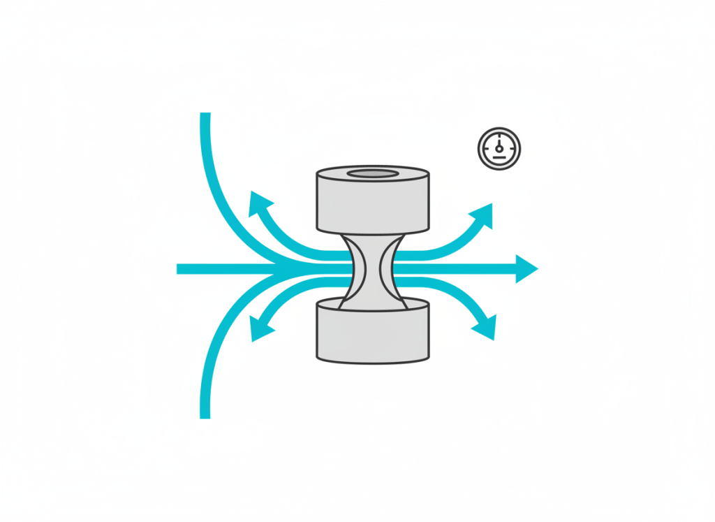
Choke management is one of the few levers a production engineer can pull without a workover rig — open the bean and rate goes up, close it and drawdown eases off. That makes it the front line for managing sand production, controlling water or gas breakthrough, and keeping a well inside its allowable drawdown while completions and reservoir teams argue about the longer-term plan. Knowing exactly what rate a given choke setting will deliver, before you open the manifold, turns that lever from a guess into a decision.

Prerequisites

• Upstream (wellhead) flowing pressure, P_wh — psia. Example: 800 psia.
• Choke bean size, D — in 64ths of an inch. Example: 32/64″ (½ inch).
• Producing gas-liquid ratio, GLR — scf/bbl. Example: 500 scf/bbl.
• Confirmation that flow through the choke is critical (sonic) — downstream pressure at or below roughly 70% of P_wh. The correlations below only hold under critical flow.
• Python 3, no libraries required for the calculation itself.

Why “Critical Flow” Is the Whole Ballgame

When a downstream pressure change can no longer be felt upstream of the choke — because the fluid is already moving as fast as the pressure drop allows — the flow is critical, or sonic. Practically, that happens whenever the downstream (flowline) pressure is below about 70% of the upstream wellhead pressure. Under that condition, flow rate depends only on upstream conditions: P_wh, choke size, and GLR. That’s the regime the empirical correlations below were built for, and it’s why they’re so widely used — one clean equation, three inputs, no iteration.

Step 1: The Governing Equation

Every major critical-flow choke correlation takes the same shape — only the three constants change:

q_L = (P_wh × D^n) / (C × GLR^m)

Where q_L is liquid rate in bbl/day, P_wh is upstream pressure in psia, D is choke size in 64ths of an inch, and GLR is in scf/bbl. Four correlations, published between the 1950s and 1960s and still the field standard today:

Correlation	C	n (choke exponent)	m (GLR exponent)
Gilbert	10.00	1.89	0.546
Ros	17.40	2.00	0.500
Baxendell	9.56	1.93	0.546
Achong	3.82	1.88	0.650

Step 2: Work the Numbers by Hand

Take a well flowing at P_wh = 800 psia through a 32/64″ choke with GLR = 500 scf/bbl. Using the Gilbert correlation:

q_L = (800 × 32^1.89) / (10.00 × 500^0.546)
    = (800 × 699.4) / (10.00 × 29.76)
    = 559,520 / 297.6
    ≈ 1,880 bbl/d

Run the exact same inputs through the other three correlations and you get a real spread — which is the point of showing all four rather than picking a favorite:

Correlation	Predicted rate (bbl/d)
Gilbert	1,880
Ros	2,106
Baxendell	2,259
Achong	2,491

That’s a 33% spread between the lowest and highest estimate for the exact same choke, pressure, and GLR. None of the four is universally “right” — each was fit to a different set of fields. The professional move is to calibrate against your own well tests: run a rate test at a known choke size, see which correlation lands closest, and use that one for the rest of the field.

Step 2b: See How Sensitive the Rate Really Is

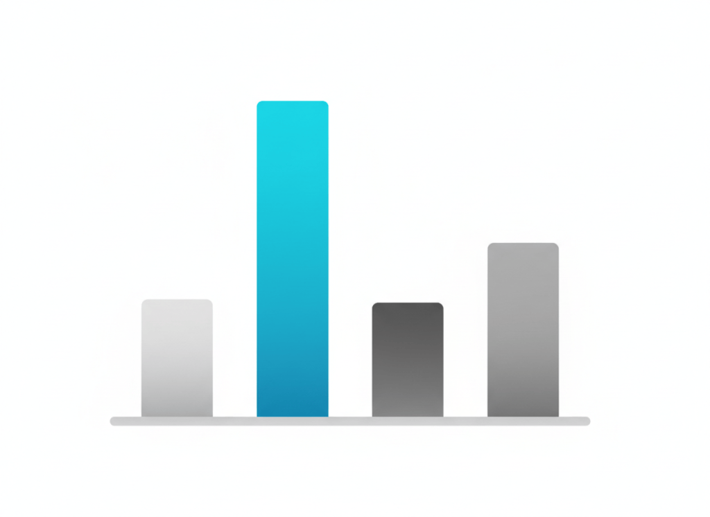
The choke-size exponent (1.89 for Gilbert) means rate is far more sensitive to bean size than to GLR. Holding P_wh = 800 psia and GLR = 500 scf/bbl fixed and stepping the choke size up from 24/64″ to 40/64″:

Choke size (64ths)	Gilbert rate (bbl/d)
24	1,092
28	1,461
32	1,880
36	2,349
40	2,867

A 25% increase in choke size (32 to 40) increases predicted rate by about 52% — the near-square relationship between diameter and area, plus the exponent above 1, compounds fast. Compare that to GLR, holding D = 32/64″ fixed:

GLR (scf/bbl)	Gilbert rate (bbl/d)
300	2,485
500	1,880
800	1,455
1,200	1,166

Rate still falls as GLR climbs, but far more gently than it rises with choke size. Practically: if you need to change rate meaningfully, the choke bean is your lever; GLR drifting up over the life of the well will erode rate steadily, but it’s rarely the variable you’re actively controlling day to day.

All four correlations above only hold for critical flow. Once the downstream pressure rises above roughly 70% of P_wh, flow becomes subcritical and rate starts depending on the downstream pressure too — a different class of model (Sachdeva-type subcritical correlations are the standard reference) is needed at that point. Treat that as a flag to re-check your flow regime, not as a reason to keep using a critical-flow number that no longer applies.

Step 3: Automate the Choke Performance Calculation in Python

Once you’ve picked (or want to compare) correlations, there’s no reason to look any of this up again. This function reproduces every number above and scales to a whole choke schedule in one call. Build it once in Python — a Jupyter notebook is the natural home for it:

CORRELATIONS = {
    "Gilbert":   (10.00, 1.89, 0.546),
    "Ros":       (17.40, 2.00, 0.500),
    "Baxendell": (9.56, 1.93, 0.546),
    "Achong":    (3.82, 1.88, 0.650),
}

def choke_rate(Pwh, D64, GLR, correlation="Gilbert"):
    """
    Pwh  : upstream (wellhead) flowing pressure, psia
    D64  : choke bean size, 64ths of an inch
    GLR  : producing gas-liquid ratio, scf/bbl
    Returns liquid rate in bbl/day under critical (sonic) flow.
    """
    C, n, m = CORRELATIONS[correlation]
    return Pwh * (D64 ** n) / (C * (GLR ** m))

for name in CORRELATIONS:
    q = choke_rate(Pwh=800, D64=32, GLR=500, correlation=name)
    print(f"{name:10s} {q:,.0f} bbl/d")

# Gilbert     1,880 bbl/d
# Ros         2,106 bbl/d
# Baxendell   2,259 bbl/d
# Achong      2,491 bbl/d

Loop that function over a range of choke sizes (say 16/64″ to 48/64″) and a handful of GLR values, drop the results into pandas, and you have a full choke performance curve — the kind of chart that used to live laminated on a clipboard, now regenerated on demand for any well.

Verify the Result

• Check the critical-flow assumption first. If your actual downstream (flowline) pressure is more than ~70% of P_wh, flow is subcritical and none of these four correlations apply — the rate now depends on downstream pressure too.
• Sanity-check against a known point. If you have even one rate test at a known choke size, run it through all four correlations and see which one comes closest before trusting any of them on a new choke setting.
• Watch the units. D is in 64ths of an inch (a ½” bean is D = 32, not 0.5), and GLR is scf/bbl, not Mscf/bbl — mixing those up is the single most common error in a hand calculation.

Common Pitfalls

• Applying a critical-flow correlation to subcritical flow. Always check the downstream/upstream pressure ratio before trusting the number.
• Picking one correlation and never revisiting it. A 33% spread between correlations on identical inputs means the “right” one is field-specific, not universal.
• Ignoring erosional velocity limits. A choke sized purely for rate can still push velocity past safe erosional limits in the downstream piping — always cross-check against an erosional velocity screen.
• Treating GLR as a fixed input. GLR drifts as reservoir pressure declines and gas breaks through; a choke schedule built on day-one GLR can be quietly wrong a year later if nobody updates the number.

Once you know the rate a given choke will deliver, the natural next question is whether the surface piping downstream can handle it without eroding — see the API RP 14E erosional velocity check. If the well is gas-dominated rather than oil, the choke setting also interacts with liquid loading risk, and for the full outflow picture, this feeds directly into a nodal analysis model.