

By Saad Iqbal
A corrosion technician pulls an ultrasonic thickness reading off a production header elbow and finds it’s lost 40% of its wall in under three years — on a line that was sized, on paper, for the flow rate. Nothing was wrong with the metallurgy. The problem was velocity: somewhere between the well test data and the pipe spec, nobody checked the two-phase mixture velocity against the erosional limit in API RP 14E. That single check, run at design time, would have caught it. It takes about five minutes by hand and about five lines in Python, and this tutorial walks through both.
Erosional velocity is the maximum safe velocity for a two-phase (gas-liquid) stream flowing through production tubing, flowlines, or piping before entrained liquid droplets and solids start eroding the pipe wall — worst first at elbows, tees, and other flow-direction changes, which is exactly where that corroded header elbow lived. API Recommended Practice 14E gives the standard empirical limit for this, and it’s one of the first checks a facilities or production engineer runs when sizing a new flowline or diagnosing unexplained erosion on an existing one.
Prerequisites
- Python 3.8 or newer, or a notebook environment (python.org or Jupyter)
- No external packages needed for the core calculation — only the built-in
mathmodule - Matplotlib installed only if you want to reproduce the C-factor comparison chart (
pip install matplotlib) - Flowing pressure and temperature at the point of interest, gas and liquid specific gravity, producing gas-liquid ratio (GLR), gas z-factor, and the pipe ID you’re checking
- A working definition of your service type — continuous non-corrosive, continuous corrosive/erosive with corrosion control, or intermittent service — since each carries a different API RP 14E C-factor
Step 1: Understand why elbows and tees fail first
In a straight run of pipe, a two-phase stream flows roughly parallel to the wall and erosion is comparatively slow. At an elbow or tee, the flow direction changes and entrained liquid droplets — and any solids in the stream, sand in particular — are flung against the outer wall of the bend by momentum, striking it at an angle instead of sliding past it. That impingement is what actually removes metal, and it’s why erosion damage on a production system shows up disproportionately at elbows, reducers, and tees rather than uniformly along the pipe run. The erosional velocity limit exists specifically to keep mixture velocity low enough that this impingement stays within an acceptable, slow rate rather than accelerating into the kind of wall loss that takes a header elbow from spec to failure in a few years.
Why it matters: if you’re troubleshooting unexplained erosion on an existing system, checking mixture velocity at every elbow and tee — not just at a representative straight-run point — is usually how you find which specific fittings are actually at risk, since velocity and hence erosion risk can vary along a line as pressure drops and the gas phase expands.

Step 2: Gather the inputs and pick the right C-factor
API RP 14E’s erosional velocity equation needs the flowing pressure, temperature, gas and liquid specific gravity, producing gas-liquid ratio, and the gas z-factor at flowing conditions — all standard well test outputs. The one judgment call is the empirical constant C, which sets how conservative the limit is for your service:
- C = 100 for continuous service, the standard default for most producing wells and flowlines
- C = 125 for continuous service where corrosion is controlled — by inhibitor injection, corrosion-resistant alloy, or a corrosion coating
- C = 150-200 for intermittent service, such as pigging lines or well test lines that don’t flow continuously, where a somewhat higher erosion rate is tolerable given the reduced exposure time
Why it matters: picking C = 100 when the line is actually running clean, corrosion-controlled service leaves easy velocity headroom on the table and can force an oversized, more expensive flowline; picking C = 125 or higher on a line without real corrosion control understates erosion risk. The C-factor is a design decision, not just a lookup — document which one you used and why.
Step 3: The governing equation
API RP 14E’s erosional velocity limit is:
Ve = C / √(ρm)
where Ve is erosional velocity in ft/s, C is the empirical constant from Step 2, and ρm is the two-phase mixture density in lb/ft³ at flowing conditions. Mixture density itself comes from a standard oilfield-units mass-balance form:
ρm = (12409 × Sl × P + 2.7 × R × Sg × P) / (198.7 × P + R × T × Z)
where Sl and Sg are liquid and gas specific gravity (water = 1.0, air = 1.0), P is flowing pressure in psia, R is the producing gas-liquid ratio in scf/bbl, T is flowing temperature in °R, and Z is the gas compressibility factor at flowing conditions. To compare against your actual line, you also need actual mixture velocity — which API RP 14E doesn’t hand you a companion formula for, so it has to come from first-principles continuity: total mass flow rate divided by mixture density divided by pipe cross-sectional area. The well is within the erosional limit whenever actual mixture velocity stays below Ve.
Step 4: Work a real example by hand first
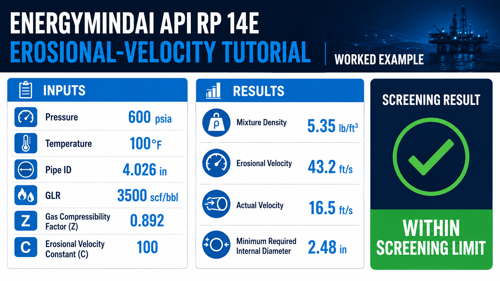
Take a well flowing at P = 600 psia, T = 100°F, through 4-1/2 inch tubing with an actual ID of 4.026 in, gas specific gravity Sg = 0.70, liquid specific gravity Sl = 0.81, producing GLR = 3,500 scf/bbl, gas z-factor Z = 0.892 at flowing conditions, gas rate of 5.0 MMscf/d, and continuous non-corrosive service (C = 100).
Mixture density: ρm = (12,409 × 0.81 × 600 + 2.7 × 3,500 × 0.70 × 600)/(198.7 × 600 + 3,500 × 560 × 0.892) ≈ 5.35 lb/ft³. Erosional velocity: Ve = 100/√5.35 ≈ 43.2 ft/s.
For actual mixture velocity, convert gas rate to liquid rate via the GLR (5,000,000 scf/d ÷ 3,500 scf/bbl ≈ 1,429 bbl/d), find total mass flow rate (gas mass + liquid mass per day), divide by mixture density to get actual volumetric flow, then divide by the 4.026 in tubing’s cross-sectional area (0.0884 ft²). That works out to an actual mixture velocity of roughly 16.5 ft/s — comfortably below the 43.2 ft/s erosional limit, so this well is within its erosional velocity limit with meaningful margin. Working backward, the minimum tubing ID that would still keep this same flow right at the erosional limit is about 2.48 in — useful context for how much oversizing margin this particular string actually has.
Step 5: Automate it in Python so you can check every line in your system
Checking one line by hand is fine once. Checking every flowline, header, and tubing string across a facility — especially after a rate change or a new well tie-in — is exactly the kind of repetitive numeric check Python is built for:
import math

def erosional_check(P, T_F, Sg, Sl, R, Z, C, Qg_mmscfd, d_in):
    """API RP 14E erosional velocity check.
    P: flowing pressure, psia. T_F: flowing temp, deg F.
    Sg, Sl: gas/liquid specific gravity. R: GLR, scf/bbl.
    Z: gas z-factor. C: API RP 14E constant (100/125/150-200).
    Qg_mmscfd: gas rate, MMscf/d. d_in: pipe ID, inches.
    Returns (mixture density lb/ft3, erosional velocity ft/s,
             actual mixture velocity ft/s, min ID for this Ve, in)."""
    T = T_F + 460
    rho_m = (12409 * Sl * P + 2.7 * R * Sg * P) / (198.7 * P + R * T * Z)
    Ve = C / math.sqrt(rho_m)

    Qg_scfd = Qg_mmscfd * 1e6
    Qliq_bpd = Qg_scfd / R
    mdot = Qg_scfd * 0.0765 * Sg + Qliq_bpd * 350.4 * Sl   # lbm/day
    A = math.pi / 4 * (d_in / 12) ** 2                      # ft^2
    q_actual_ft3s = mdot / rho_m / 86400
    Vm = q_actual_ft3s / A
    d_min_in = math.sqrt(4 * q_actual_ft3s / (math.pi * Ve)) * 12
    return rho_m, Ve, Vm, d_min_in

rho_m, Ve, Vm, d_min = erosional_check(
    P=600, T_F=100, Sg=0.70, Sl=0.81, R=3500, Z=0.892,
    C=100, Qg_mmscfd=5.0, d_in=4.026
)
print(f"Mixture density:   {rho_m:.2f} lb/ft3")
print(f"Erosional velocity: {Ve:.1f} ft/s")
print(f"Actual velocity:    {Vm:.1f} ft/s")
print(f"Min ID at Ve limit: {d_min:.2f} in")

# >> Mixture density:   5.35 lb/ft3
# >> Erosional velocity: 43.2 ft/s
# >> Actual velocity:    16.5 ft/s
# >> Min ID at Ve limit: 2.48 in
The printed values match the hand calculation in Step 4 exactly — that’s your sanity check that the code is doing what the equations say. From here, looping this function over a CSV of every line in your system (with each line’s own pressure, GLR, and diameter) turns a one-off design check into a standing erosion-risk audit you can rerun every time production rates shift.
It’s also worth seeing how much headroom the C-factor choice actually buys you, since that’s the one input in this whole calculation that’s a judgment call rather than a measurement:

Moving from C = 100 to C = 125 for corrosion-controlled service raises the erosional limit by 25% for the same mixture density — real design margin, but only defensible if the corrosion control is actually in place and maintained. If you’re also running a real-gas z-factor calculation for a nitrogen job on the same well, that same z-factor correlation plugs directly into the mixture density equation here. And if erosional velocity comes back marginal or exceeded on an existing line, the next step is usually the kind of wall-thickness and remaining-life check covered in our pipeline corrosion reporting tutorial.
Expected result and how to verify it
Running the function above on the worked example should return a mixture density of 5.35 lb/ft³, an erosional velocity of 43.2 ft/s, an actual mixture velocity of 16.5 ft/s, and a minimum ID of 2.48 in — confirming the well is comfortably within its erosional limit. As a sanity check, typical erosional velocities for oilfield production conditions usually fall in the 30-100 ft/s range depending on mixture density and C-factor; if your result is far outside that band, check that pressure is in psia (not psig) and GLR is in scf/bbl (not scf/STB confused with a different basis), since those unit mismatches are the most common source of an order-of-magnitude error here.
Common pitfalls
- Applying one C-factor to a whole system. A gathering line with sand production or an unlined elbow downstream of a choke may need the conservative C = 100 even if the rest of the facility runs corrosion-controlled service at C = 125 — check the C-factor fitting by fitting, not facility-wide.
- Checking mixture velocity only at the meter run. Velocity changes along a line as pressure drops and gas expands — the highest-risk point is often near the downstream end of a long flowline, not where the flow was originally measured.
- Ignoring solids production when picking C. API RP 14E’s C-factor framework was developed primarily for liquid droplet erosion; a well producing sand needs a materially more conservative velocity limit than the standard table implies, regardless of which C-factor otherwise applies.
None of this replaces a proper erosion/corrosion engineering study for a new facility design — but as a five-minute check before a line goes into service, or a five-line script run across every fitting in an existing system, it’s usually enough to catch the kind of oversight that turned a routine header elbow into a 40%-wall-loss surprise.
