Best AI Decline Curve Analysis Tools for 2026

By Saad Iqbal

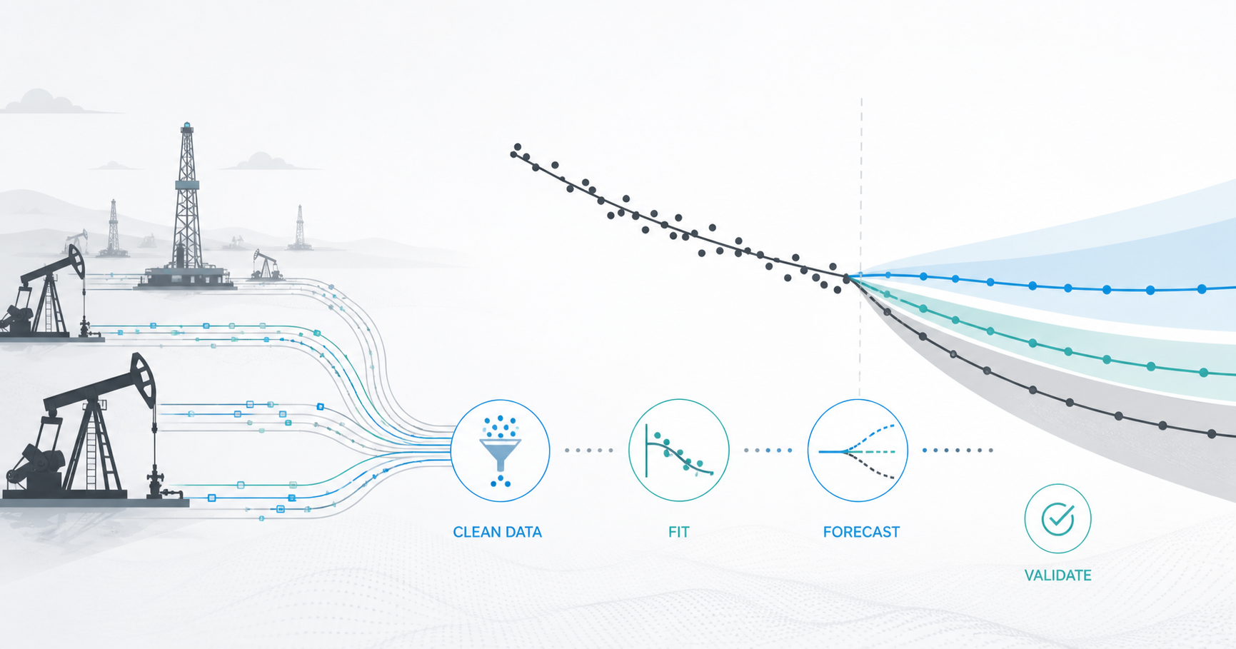
AI decline curve analysis tools can clean production histories, fit Arps models, screen uncertainty and produce auditable forecasts without hiding the engineering assumptions.

It’s 11 p.m. and the reserves report is due in the morning. You’ve got 40 wells open in a spreadsheet, each with its own tab, each with a hand-picked “b” exponent that seemed reasonable three months ago and now looks wrong against the last two months of production. You nudge qi, drag the trendline, eyeball the fit, and move to the next tab. By well 25 you’re not really looking anymore — you’re pattern-matching to whatever got you out of the last well. This is decline curve analysis the way most of the industry still does it, and it is exactly the kind of repetitive, error-prone task that AI and automation tools were built to remove.

Decline curve analysis, or DCA, is one of the oldest tools in petroleum engineering and still one of the most load-bearing: it drives reserves bookings, type curves, acquisition valuations, and the production forecasts that show up in board decks. It’s also, in most shops, still done by hand in Excel. In this post we’ll walk through what DCA actually solves, why the manual version stops scaling somewhere around well number 30, and compare the real, currently available AI decline curve analysis tools — Novi Labs, Enverus, ARIES, and a Python-based open-source route — so you can pick the right one for your team.

What Decline Curve Analysis Actually Solves

Every producing well declines. The question DCA answers is: how fast, and following what shape? The workhorse is the Arps equation, published by J.J. Arps in 1945 and still the industry standard for empirical production forecasting:

q(t) = qi · (1 + b·Di·t)^(-1/b)

• q(t) — production rate at time t
• qi — initial production rate
• Di — initial decline rate
• b — the decline exponent, which controls the curve’s shape

The value of b is what separates the three named decline types: exponential (b = 0, a constant percentage decline, common late in a well’s life), hyperbolic (0 < b < 1, the typical shape for unconventional wells in their first years), and harmonic (b = 1, the slowest-declining and least common case). Get b wrong and your estimated ultimate recovery (EUR) can swing by double digits — which is exactly why this isn’t a “close enough” exercise when it feeds a reserves audit.

Why Manual DCA Breaks Down Past a Handful of Wells

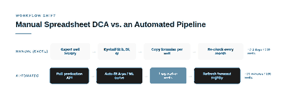
Fitting one well by hand is fine. Fitting one well correctly, with a defensible b and Di that a reserves auditor won’t flag, takes real judgment — and that judgment doesn’t scale linearly. At 10 wells, manual DCA in Excel is annoying. At 100 wells, refreshed monthly, it becomes a full-time job that nobody has time to actually do well, so shortcuts creep in: last quarter’s b gets copied forward, outlier wells get eyeballed instead of properly re-fit, and nobody catches the well that started producing water and needs a completely different curve.

The tools below don’t replace engineering judgment — they replace the repetitive part, so your judgment goes toward the wells that actually need it (the outliers, the newly online wells, the ones where the fit genuinely looks wrong) instead of being spread thin across everything.

Four Ways to Automate Decline Curve Analysis in 2026

These four cover the realistic range of options, from fully managed machine learning platforms to a free Python library you run yourself.

1. Novi Labs — machine learning built for unconventional wells

Novi Labs is a cloud-based, code-free machine learning platform purpose-built for oil and gas production forecasting. Rather than fitting a single Arps curve per well, its Model Engine forecasts the full production curve — capturing peak rate, the shift into decline, and late-time behavior — and it does this using transparent, white-box models rather than a black box, so you can inspect what drove a given forecast. It automatically identifies analog wells, handles unit conversion and data normalization, and can forecast producing wells, undrilled locations, or hypothetical completion designs. For teams managing large unconventional portfolios where re-forecasting has to happen on a schedule, this is the most “hands-off” of the four options here.

Best for: shale/unconventional portfolios with dozens to thousands of wells that need scheduled, auditable re-forecasts.

2. Enverus — decline curve analytics tied to asset evaluation

Enverus builds decline curve and type-curve analysis directly into its broader analytics platform, which is the point: your DCA output isn’t a standalone spreadsheet, it’s connected to acreage benchmarking, asset evaluation, and production forecast solutions used across A&D (acquisition and divestiture) workflows. If your DCA needs to talk to a reserves or deal team that already lives in Enverus for offset-well benchmarking, keeping the forecasting in the same platform avoids a lot of re-exporting.

Best for: reserves and A&D teams who need DCA results to plug straight into asset valuation and benchmarking.

3. ARIES — decline forecasts wired to reserves and economics

ARIES, now part of Halliburton’s DecisionSpace 365 Enterprise suite, is a petroleum economics and reserves software package where decline forecasting isn’t the end product — it’s the input to a reserves booking and economic evaluation. If your team’s actual deliverable is a reserves report or an economic run rather than a chart, ARIES keeps the decline curve and the dollars in one place instead of two.

Best for: reserves engineers who need the decline forecast to flow directly into economic evaluation and bookings.

4. Python + petropt — free, scriptable, and fully transparent

If you don’t need a managed platform, Python with the open-source petropt library will fit exponential, hyperbolic, and harmonic Arps decline in a handful of lines, with no license cost and no vendor lock-in. It’s MIT-licensed, so you can wire it into whatever internal pipeline or dashboard you already have. The tradeoff is that you’re the QC layer — there’s no built-in analog-well logic or reserves workflow, just the math, cleanly implemented.

import petropt as pp
import pandas as pd

# production history: date, oil rate (bopd)
prod = pd.read_csv("well_123_production.csv")

# fit a hyperbolic Arps decline
fit = pp.arps.fit(
    t=prod["days_on"],
    q=prod["oil_bopd"],
    decline_type="hyperbolic"
)

print(fit.qi, fit.di, fit.b)
forecast = pp.arps.forecast(fit, days=3650)  # 10-year forecast

Best for: engineers comfortable in Python who want batch runs, custom QC rules, or to plug decline forecasts into an internal dashboard.

Common Pitfalls Even Automated DCA Won’t Fix for You

Automating the curve fit removes the tedium, not the engineering judgment. A few things still need a human to catch:

• Bad data in, confident forecast out. A choked-back well, a shut-in period, or a metering error will still get fit smoothly by any of these tools — smoothly and wrong. Always sanity-check the raw production trace before trusting the fit.
• b > 1 forecasts that never terminate. A hyperbolic fit with an unconstrained b can predict decades of production at implausibly high rates. Most platforms let you cap b or switch to exponential decline past a certain time — use it.
• Water breakthrough and artificial lift changes. A well that goes from natural flow to gas lift, or starts making significant water, often needs a fresh curve rather than a continuation of the old one. No automated tool knows this happened unless you tell it or it’s watching the water cut trend directly.
• Type curves built on too few analogs. Machine-learning forecasts for undrilled locations are only as good as the analog wells behind them — a handful of wells from a different bench or spacing pattern will quietly bias the result.

How to Choose the Right Tool for Your Team

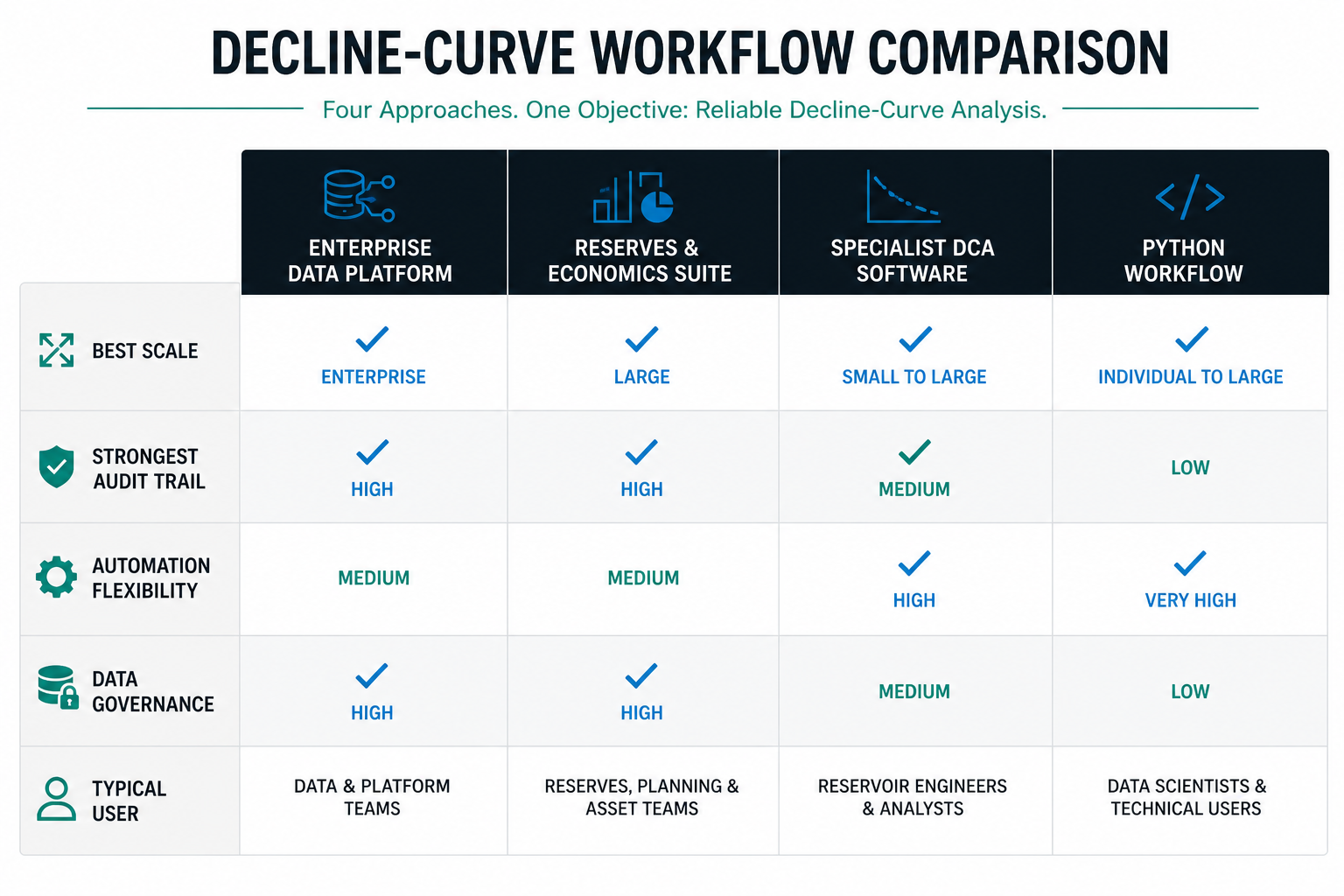
The honest answer is that the four tools above aren’t really competing for the same job:

• If the deliverable is a reserves report — start with ARIES or Enverus, since the forecast needs to flow into economics and bookings anyway.
• If you’re managing a large unconventional portfolio and need scheduled, defensible re-forecasts without a reserves engineer touching every well — Novi Labs’ machine learning approach scales better than any manual or semi-manual method.
• If you need something today, for free, and you’re comfortable writing code — Python plus petropt gets you a correct Arps fit in an afternoon.
• If your team already lives in one of these platforms for offset-well data or economics, the marginal cost of also doing DCA there is usually lower than standing up a second tool.

Whichever route you pick, the underlying math doesn’t change — the Arps equation, the three decline shapes, and the discipline of re-checking b against fresh production data. The tools just decide how much of the repetitive fitting you do by hand versus how much gets done for you.

Want to see nodal analysis get the same automation treatment? Read our related tutorial on automating IPR-VLP nodal analysis in Python, or compare reservoir-scale forecasting tools in Best AI Reservoir Simulation Tools for 2026.