
By Saad Iqbal
A production engineer gets a single pressure build-up test back from the field: reservoir pressure, one flowing bottomhole pressure, one flow rate. Three numbers. From that alone, the completions team wants to know whether the well can support a bigger choke, whether an ESP is worth running, and what the well could flow if drawdown were pushed harder. Reaching for nodal analysis software for a quick sanity check is overkill, and guessing is worse. The fix engineers have used since 1968 is the Vogel IPR equation — a single curve-fit formula that turns one test point into a full inflow performance relationship (IPR) curve, by hand, in under five minutes.
This tutorial walks through the Vogel IPR equation step by step: what it assumes, a full worked example with real numbers, and a Python function so you never have to repeat the arithmetic by hand again.
What the Vogel IPR Equation Actually Does
The inflow performance relationship (IPR) describes how much a well will flow (qo) at a given flowing bottomhole pressure (Pwf). For an undersaturated oil well above the bubble point, that relationship is a straight line (the productivity index, PI, method). Below the bubble point, free gas comes out of solution in the reservoir, relative permeability to oil drops, and the IPR curve bends — a straight-line PI model badly overstates how much the well can flow at low Pwf.
In 1968, Vogel published an empirical curve fit for solution-gas-drive reservoirs below the bubble point, built from reservoir simulation runs across a wide range of conditions:
qo / qo_max = 1 - 0.2 (Pwf / Pr) - 0.8 (Pwf / Pr)^2Where qo is the oil rate at flowing bottomhole pressure Pwf, Pr is the average reservoir (static) pressure, and qo_max is the Absolute Open Flow potential (AOF) — the theoretical rate if Pwf could be dropped to zero. That AOF term is the entire trick: once you know it, you can compute qo at any Pwf you want.
Prerequisites
- Tool: any calculator for the hand steps; Python 3.10+ with pandas for the automation step (no special library required).
- Inputs needed: average reservoir pressure (Pr), and one stabilized flow test point — a flowing bottomhole pressure (Pwf_test) and the matching oil rate (qo_test).
- Sample values used in this walkthrough: Pr = 2,500 psi, Pwf_test = 2,000 psi, qo_test = 300 STB/d. Swap in your own well’s numbers — the method doesn’t change.
- Applicability check: Pwf_test must be below the bubble point pressure for Vogel to apply (see the pitfalls section below).
Step 1: Gather Your Well Test Data
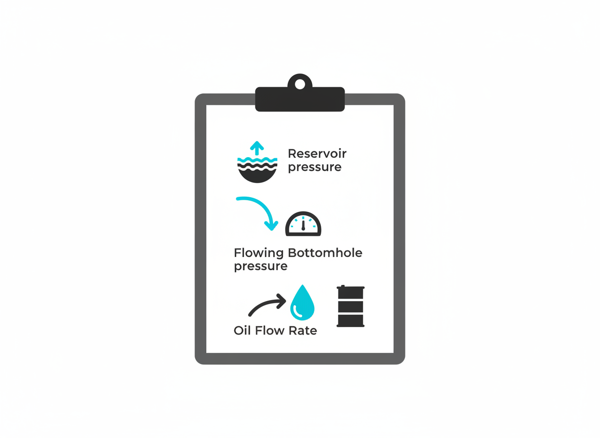
You need exactly three numbers from a single stabilized flow test: the average reservoir pressure Pr (from a build-up or the last known static survey), the flowing bottomhole pressure Pwf_test during the test (measured or calculated from wellhead pressure plus a gradient traverse), and the stabilized oil rate qo_test at that Pwf. Why it matters: every other point on the IPR curve is extrapolated from this one test, so a rushed, non-stabilized test point will throw off the whole curve — let the well stabilize before you read the rate.
For this walkthrough: Pr = 2,500 psi, Pwf_test = 2,000 psi, qo_test = 300 STB/d.
Step 2: Calculate Absolute Open Flow (AOF) with the Vogel IPR Equation
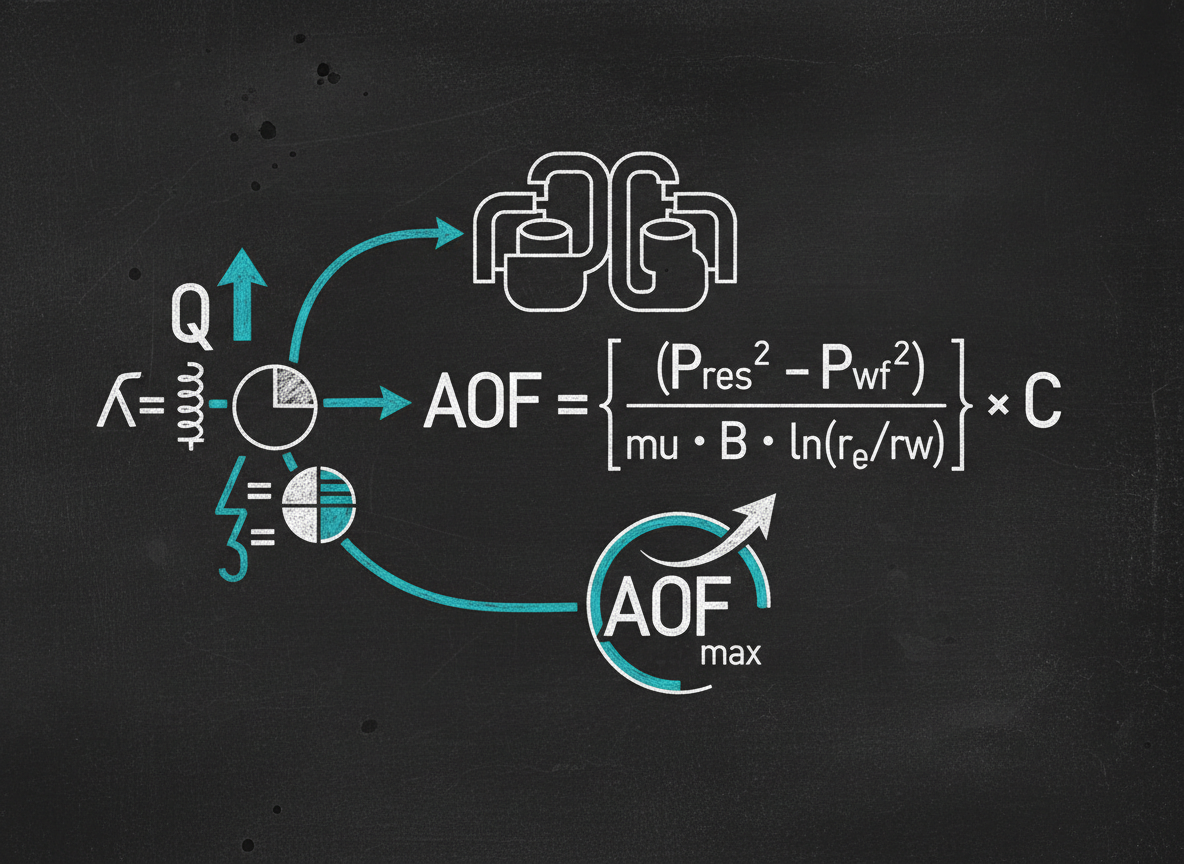
Rearrange the Vogel equation to solve for qo_max (AOF) using your one test point. Why it matters: AOF is the anchor value — get it right and the whole IPR curve follows automatically.
qo_max = qo_test / [1 - 0.2(Pwf_test/Pr) - 0.8(Pwf_test/Pr)^2]Worked example:
- Pwf_test / Pr = 2,000 / 2,500 = 0.8
- 1 − 0.2(0.8) − 0.8(0.8)² = 1 − 0.16 − 0.512 = 0.328
- qo_max = 300 / 0.328 = 914.6 STB/d
This well’s Absolute Open Flow potential is about 915 STB/d — the maximum it could theoretically flow with zero bottomhole pressure. No real well is produced at Pwf = 0, but AOF is the standard reference point engineers use to compare wells and to size future drawdown.
Step 3: Build and Plot the Full IPR Curve
With qo_max known, plug a range of Pwf values back into the original Vogel equation to generate the full curve. Why it matters: a single AOF number tells you the ceiling; the full curve is what you actually overlay against a tubing performance (outflow) curve to pick an operating point in nodal analysis.
| Pwf (psi) | Pwf/Pr | qo (STB/d) |
|---|---|---|
| 2,500 | 1.00 | 0 |
| 2,000 | 0.80 | 300.0 |
| 1,500 | 0.60 | 541.5 |
| 1,000 | 0.40 | 724.4 |
| 500 | 0.20 | 848.8 |
| 0 | 0.00 | 914.6 |
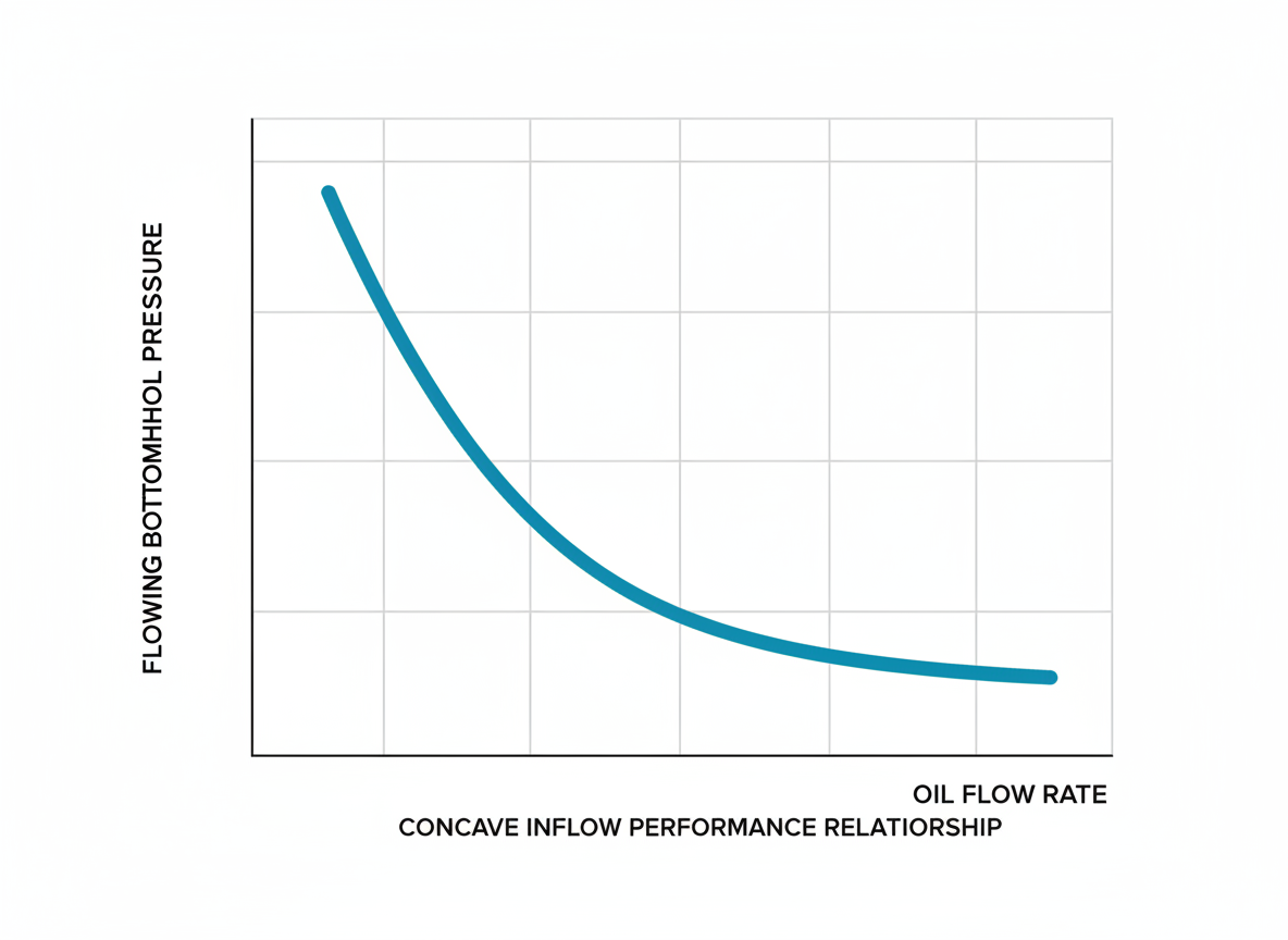
Notice the 2,000 psi row reproduces your original 300 STB/d test point exactly — that’s your built-in sanity check that the math is right. Plot Pwf (y-axis) against qo (x-axis) and you’ll see the characteristic concave-down Vogel shape: steep near AOF, flattening as Pwf approaches Pr. You can plot this by hand on graph paper, in an Excel chart, or push it into a live dashboard with Microsoft Power BI or Google Looker Studio if you’re tracking IPR curves across a multi-well pad.
Step 4: Automate It in Python So You Never Do It by Hand Again
Once you trust the hand calculation, there’s no reason to redo this arithmetic for every well, every month, as reservoir pressure declines. Here’s a small Python function that reproduces every number above — paste it into a Jupyter notebook or any script:
import pandas as pd

def vogel_aof(pr, pwf_test, qo_test):
    """Solve for Absolute Open Flow (qo_max) from one test point."""
    ratio = pwf_test / pr
    factor = 1 - 0.2 * ratio - 0.8 * ratio ** 2
    return qo_test / factor

def vogel_ipr(pr, qo_max, pwf):
    """Return oil rate at a given Pwf using Vogel's equation."""
    ratio = pwf / pr
    return qo_max * (1 - 0.2 * ratio - 0.8 * ratio ** 2)

# Inputs
pr = 2500        # reservoir pressure, psi
pwf_test = 2000  # tested flowing bottomhole pressure, psi
qo_test = 300    # tested oil rate, STB/d

qo_max = vogel_aof(pr, pwf_test, qo_test)
print(f"AOF = {qo_max:.1f} STB/d")

# Build the full IPR curve
pwf_values = [2500, 2000, 1500, 1000, 500, 0]
rates = [round(vogel_ipr(pr, qo_max, p), 1) for p in pwf_values]
ipr_curve = pd.DataFrame({"Pwf_psi": pwf_values, "qo_STBpd": rates})
print(ipr_curve)
Run it and the printed AOF and table should match Step 2 and Step 3 exactly: 914.6 STB/d, with the 2,000 psi row landing on 300.0. Point this script at a spreadsheet or a historian export and loop it across every well on a pad in seconds — something an AI coding assistant like ChatGPT or Claude can help you extend to read live well test data directly from a CSV or database.
When Should You Use Vogel Instead of a Straight-Line IPR?
Vogel’s equation is built for solution-gas-drive reservoirs producing below the bubble point, where free gas evolving in the pore space curves the IPR. Above the bubble point, oil and its dissolved gas stay in a single liquid phase, relative permeability to oil doesn’t fall off, and the straight-line productivity index (PI) method — qo = PI × (Pr − Pwf) — is both simpler and more accurate. If your test point sits above bubble point pressure, use PI; if it’s below, Vogel is the right tool.
This IPR curve is also exactly the input nodal analysis needs on the inflow side — pair it with a tubing performance (outflow) curve, such as the net lift and friction calculations in our coiled tubing friction pressure tutorial, to find where a well will actually operate.

Expected Result, Verification, and Common Pitfalls
Expected result: an AOF of roughly 915 STB/d for this example, and a six-point IPR curve running from 0 STB/d at Pwf = Pr down to AOF at Pwf = 0.
Sanity check: plug your original test point’s Pwf back into the curve — it must reproduce the original qo_test almost exactly (any Vogel implementation that doesn’t pass this check has a bug).
Common pitfalls:
- Using Vogel above the bubble point. The curve will understate well potential; check PVT data first and use the straight-line PI method instead.
- Relying on a single test point. One point fully defines the Vogel curve mathematically, but a second test point (the basis of the Fetkovich two-point method) catches a bad test and improves confidence.
- Letting the IPR go stale. Pr declines as the reservoir depletes, which shifts the whole curve down. Re-test and refresh AOF periodically rather than relying on a curve from a year-old test.
Next up: once you know what a well can inflow, the next question is what it takes to lift that fluid to surface. Read the related tutorial on calculating total dynamic head for an ESP to size the lift side of the equation.
